
CANNOT UPLOAD CHARTS AND IMAGES
Recovery without Hiring, Ten Million Fewer Full-Time Job Youth and Middle-Age Unemployment, United States International Trade, Rules, Discretionary Authorities and Slow Productivity Growth, Collapse of United States Dynamism of Income Growth and Employment Creation, World Cyclical Slow Growth and Global Recession Risk
© Carlos M. Pelaez, 2009, 2010, 2011, 2012, 2013, 2014, 2015, 2016, 2017
I Recovery without Hiring
IA1 Hiring Collapse
IA2 Labor Underutilization
ICA3 Ten Million Fewer Full-time Jobs
IA4 Theory and Reality of Cyclical Slow Growth Not Secular Stagnation: Youth and Middle-Age Unemployment
IIA United States International Trade
IIB Rules, Discretionary Authorities and Slow Productivity Growth
II IB Collapse of United States Dynamism of Income Growth and Employment Creation
III World Financial Turbulence
IIIA Financial Risks
IIIE Appendix Euro Zone Survival Risk
IIIF Appendix on Sovereign Bond Valuation
IV Global Inflation
V World Economic Slowdown
VA United States
VB Japan
VC China
VD Euro Area
VE Germany
VF France
VG Italy
VH United Kingdom
VI Valuation of Risk Financial Assets
VII Economic Indicators
VIII Interest Rates
IX Conclusion
References
Appendixes
Appendix I The Great Inflation
IIIB Appendix on Safe Haven Currencies
IIIC Appendix on Fiscal Compact
IIID Appendix on European Central Bank Large Scale Lender of Last Resort
IIIG Appendix on Deficit Financing of Growth and the Debt Crisis
IIIGA Monetary Policy with Deficit Financing of Economic Growth
IIIGB Adjustment during the Debt Crisis of the 1980s
I Recovery without Hiring. Professor Edward P. Lazear (2012Jan19) at Stanford University finds that recovery of hiring in the US to peaks attained in 2007 requires an increase of hiring by 30 percent while hiring levels increased by only 4 percent from Jan 2009 to Jan 2012. The high level of unemployment with low level of hiring reduces the statistical probability that the unemployed will find a job. According to Lazear (2012Jan19), the probability of finding a new job in early 2012 is about one third of the probability of finding a job in 2007. Improvements in labor markets have not increased the probability of finding a new job. Lazear (2012Jan19) quotes an essay coauthored with James R. Spletzer in the American Economic Review (Lazear and Spletzer 2012Mar, 2012May) on the concept of churn. A dynamic labor market occurs when a similar number of workers is hired as those who are separated. This replacement of separated workers is called churn, which explains about two-thirds of total hiring. Typically, wage increases received in a new job are higher by 8 percent. Lazear (2012Jan19) argues that churn has declined 35 percent from the level before the recession in IVQ2007. Because of the collapse of churn, there are no opportunities in escaping falling real wages by moving to another job. As this blog argues, there are meager chances of escaping unemployment because of the collapse of hiring and those employed cannot escape falling real wages by moving to another job (Section I and earlier https://cmpassocregulationblog.blogspot.com/2017/10/increasing-valuations-of-risk-financial.html). Lazear and Spletzer (2012Mar, 1) argue that reductions of churn reduce the operational effectiveness of labor markets. Churn is part of the allocation of resources or in this case labor to occupations of higher marginal returns. The decline in churn can harm static and dynamic economic efficiency. Losses from decline of churn during recessions can affect an economy over the long-term by preventing optimal growth trajectories because resources are not used in the occupations where they provide highest marginal returns. Lazear and Spletzer (2012Mar 7-8) conclude that: “under a number of assumptions, we estimate that the loss in output during the recession [of 2007 to 2009] and its aftermath resulting from reduced churn equaled $208 billion. On an annual basis, this amounts to about .4% of GDP for a period of 3½ years.”
There are two additional facts discussed below: (1) there are about ten million fewer full-time jobs currently than before the recession of 2008 and 2009; and (2) the extremely high and rigid rate of youth unemployment is denying an early start to young people ages 16 to 24 years while unemployment of ages 45 years or over has swelled. There are four subsections. IA1 Hiring Collapse provides the data and analysis on the weakness of hiring in the United States economy. IA2 Labor Underutilization provides the measures of labor underutilization of the Bureau of Labor Statistics (BLS). Statistics on the decline of full-time employment are in IA3 Ten Million Fewer Full-time Jobs. IA4 Theory and Reality of Cyclical Slow Growth Not Secular Stagnation: Youth and Middle-Age Unemployment provides the data on high unemployment of ages 16 to 24 years and of ages 45 years or over.
IA1 Hiring Collapse. An important characteristic of the current fractured labor market of the US is the closing of the avenue for exiting unemployment and underemployment normally available through dynamic hiring. Another avenue that is closed is the opportunity for advancement in moving to new jobs that pay better salaries and benefits again because of the collapse of hiring in the United States. Those who are unemployed or underemployed cannot find a new job even accepting lower wages and no benefits. The employed cannot escape declining inflation-adjusted earnings because there is no hiring. The objective of this section is to analyze hiring and labor underutilization in the United States.
Blanchard and Katz (1997, 53 consider an appropriate measure of job stress:
“The right measure of the state of the labor market is the exit rate from unemployment, defined as the number of hires divided by the number unemployed, rather than the unemployment rate itself. What matters to the unemployed is not how many of them there are, but how many of them there are in relation to the number of hires by firms.”
The natural rate of unemployment and the similar NAIRU are quite difficult to estimate in practice (Ibid; see Ball and Mankiw 2002).
The Bureau of Labor Statistics (BLS) created the Job Openings and Labor Turnover Survey (JOLTS) with the purpose that (http://www.bls.gov/jlt/jltover.htm#purpose):
“These data serve as demand-side indicators of labor shortages at the national level. Prior to JOLTS, there was no economic indicator of the unmet demand for labor with which to assess the presence or extent of labor shortages in the United States. The availability of unfilled jobs—the jobs opening rate—is an important measure of tightness of job markets, parallel to existing measures of unemployment.”
The BLS collects data from about 16,000 US business establishments in nonagricultural industries through the 50 states and DC. The data are released monthly and constitute an important complement to other data provided by the BLS (see also Lazear and Spletzer 2012Mar, 6-7).
There is socio-economic stress in the combination of adverse events and cyclical performance:
- Mediocre economic growth below potential and long-term trend, resulting in idle productive resources with GDP two trillion dollars below trend (https://cmpassocregulationblog.blogspot.com/2017/10/dollar-revaluation-and-increase-of.html and earlier https://cmpassocregulationblog.blogspot.com/2017/10/destruction-of-household-nonfinancial.html). US GDP grew at the average rate of 3.2 percent per year from 1929 to 2016, with similar performance in whole cycles of contractions and expansions, but only at 1.3 percent per year on average from 2007 to 2016. GDP in IIIQ2017 is 14.2 percent lower than what it would have been had it grown at trend of 3.0 percent
- Private fixed investment stagnating at cumulative increase of 12.5 percent in the entire cycle from IVQ2007 to IIIQ2017 (https://cmpassocregulationblog.blogspot.com/2017/10/dollar-revaluation-and-increase-of.html and earlier https://cmpassocregulationblog.blogspot.com/2017/10/destruction-of-household-nonfinancial.html)
- Twenty one million or 12.5 percent of the effective labor force unemployed or underemployed in involuntary part-time jobs with stagnating or declining real wages (https://cmpassocregulationblog.blogspot.com/2017/11/unchanged-fomc-policy-rate-gradual.html and earlier https://cmpassocregulationblog.blogspot.com/2017/10/twenty-one-million-unemployed-or.html and earlier https://cmpassocregulationblog.blogspot.com/2017/09/twenty-two-million-unemployed-or.html and earlier https://cmpassocregulationblog.blogspot.com/2017/08/data-dependent-monetary-policy-with.html and earlier https://cmpassocregulationblog.blogspot.com/2017/07/rising-yields-twenty-two-million.html and earlier https://cmpassocregulationblog.blogspot.com/2017/06/twenty-two-million-unemployed-or.html and earlier https://cmpassocregulationblog.blogspot.com/2017/05/twenty-two-million-unemployed-or.html and earlier https://cmpassocregulationblog.blogspot.com/2017/04/twenty-three-million-unemployed-or.html and earlier https://cmpassocregulationblog.blogspot.com/2017/03/increasing-interest-rates-twenty-four.html and earlier https://cmpassocregulationblog.blogspot.com/2017/02/twenty-six-million-unemployed-or.html and earlier http://cmpassocregulationblog.blogspot.com/2017/01/twenty-four-million-unemployed-or.html and earlier http://cmpassocregulationblog.blogspot.com/2016/12/rising-yields-and-dollar-revaluation.html and earlier http://cmpassocregulationblog.blogspot.com/2016/11/the-case-for-increase-in-federal-funds.html and earlier http://cmpassocregulationblog.blogspot.com/2016/10/twenty-four-million-unemployed-or.html and earlier http://cmpassocregulationblog.blogspot.com/2016/09/interest-rates-and-valuations-of-risk.html and earlier http://cmpassocregulationblog.blogspot.com/2016/08/global-competitive-easing-or.html and earlier http://cmpassocregulationblog.blogspot.com/2016/07/fluctuating-valuations-of-risk.html and earlier http://cmpassocregulationblog.blogspot.com/2016/06/financial-turbulence-twenty-four.html and earlier http://cmpassocregulationblog.blogspot.com/2016/05/twenty-four-million-unemployed-or.html and earlier http://cmpassocregulationblog.blogspot.com/2016/04/proceeding-cautiously-in-monetary.html and earlier http://cmpassocregulationblog.blogspot.com/2016/03/twenty-five-million-unemployed-or.html and earlier http://cmpassocregulationblog.blogspot.com/2016/02/fluctuating-risk-financial-assets-in.html and earlier http://cmpassocregulationblog.blogspot.com/2016/01/weakening-equities-with-exchange-rate.html and earlier (http://cmpassocregulationblog.blogspot.com/2015/12/liftoff-of-fed-funds-rate-followed-by.html and earlier http://cmpassocregulationblog.blogspot.com/2015/11/live-possibility-of-interest-rates.html and earlier http://cmpassocregulationblog.blogspot.com/2015/10/labor-market-uncertainty-and-interest.html and earlier http://cmpassocregulationblog.blogspot.com/2015/09/interest-rate-policy-dependent-on-what.html and earlier http://cmpassocregulationblog.blogspot.com/2015/08/fluctuating-risk-financial-assets.html and earlier http://cmpassocregulationblog.blogspot.com/2015/07/turbulence-of-financial-asset.html)
- Stagnating real disposable income per person or income per person after inflation and taxes (https://cmpassocregulationblog.blogspot.com/2017/11/unchanged-fomc-policy-rate-gradual.html and earlier https://cmpassocregulationblog.blogspot.com/2017/10/twenty-one-million-unemployed-or.html and earlier https://cmpassocregulationblog.blogspot.com/2017/09/twenty-two-million-unemployed-or.html and earlier https://cmpassocregulationblog.blogspot.com/2017/08/data-dependent-monetary-policy-with.html and earlier https://cmpassocregulationblog.blogspot.com/2017/07/rising-yields-twenty-two-million.html and earlier https://cmpassocregulationblog.blogspot.com/2017/06/twenty-two-million-unemployed-or.html and earlier https://cmpassocregulationblog.blogspot.com/2017/05/twenty-two-million-unemployed-or.html and earlier https://cmpassocregulationblog.blogspot.com/2017/04/twenty-three-million-unemployed-or.html and earlier https://cmpassocregulationblog.blogspot.com/2017/03/rising-valuations-of-risk-financial.html and earlier https://cmpassocregulationblog.blogspot.com/2017/02/twenty-six-million-unemployed-or.html and earlier http://cmpassocregulationblog.blogspot.com/2017/01/twenty-four-million-unemployed-or.html and earlier http://cmpassocregulationblog.blogspot.com/2016/12/rising-yields-and-dollar-revaluation.html and earlier http://cmpassocregulationblog.blogspot.com/2016/12/mediocre-cyclical-united-states.html and earlier http://cmpassocregulationblog.blogspot.com/2016/12/rising-yields-and-dollar-revaluation.html and earlier http://cmpassocregulationblog.blogspot.com/2016/11/the-case-for-increase-in-federal-funds.html and earlier http://cmpassocregulationblog.blogspot.com/2016/11/the-case-for-increase-in-federal-funds.html and earlier http://cmpassocregulationblog.blogspot.com/2016/10/twenty-four-million-unemployed-or.html and earlier http://cmpassocregulationblog.blogspot.com/2016/09/interest-rates-and-valuations-of-risk.html and earlier http://cmpassocregulationblog.blogspot.com/2016/08/global-competitive-easing-or.html and earlier (http://cmpassocregulationblog.blogspot.com/2016/07/financial-asset-values-rebound-from.html and earlier http://cmpassocregulationblog.blogspot.com/2016/06/financial-turbulence-twenty-four.html and earlier http://cmpassocregulationblog.blogspot.com/2016/05/twenty-four-million-unemployed-or.html and earlier http://cmpassocregulationblog.blogspot.com/2016/04/proceeding-cautiously-in-monetary.html and earlier http://cmpassocregulationblog.blogspot.com/2016/03/twenty-five-million-unemployed-or.html and earlier http://cmpassocregulationblog.blogspot.com/2016/03/twenty-five-million-unemployed-or.html and earlier http://cmpassocregulationblog.blogspot.com/2016/02/fluctuating-risk-financial-assets-in.html and earlier http://cmpassocregulationblog.blogspot.com/2015/12/dollar-revaluation-and-decreasing.html and earlier http://cmpassocregulationblog.blogspot.com/2015/11/dollar-revaluation-constraining.html and earlier http://cmpassocregulationblog.blogspot.com/2015/11/dollar-revaluation-constraining.html and earlier http://cmpassocregulationblog.blogspot.com/2015/11/live-possibility-of-interest-rates.html and earlier http://cmpassocregulationblog.blogspot.com/2015/10/labor-market-uncertainty-and-interest.html and earlier http://cmpassocregulationblog.blogspot.com/2015/09/interest-rate-policy-dependent-on-what.html and earlier http://cmpassocregulationblog.blogspot.com/2015/08/fluctuating-risk-financial-assets.html and earlier http://cmpassocregulationblog.blogspot.com/2015/06/international-valuations-of-financial.html and earlier http://cmpassocregulationblog.blogspot.com/2015/06/higher-volatility-of-asset-prices-at.html and earlier http://cmpassocregulationblog.blogspot.com/2015/05/dollar-devaluation-and-carry-trade.html and earlier http://cmpassocregulationblog.blogspot.com/2015/04/volatility-of-valuations-of-financial.html)
- Depressed hiring that does not afford an opportunity for reducing unemployment/underemployment and moving to better-paid jobs (Section I and earlier https://cmpassocregulationblog.blogspot.com/2017/10/increasing-valuations-of-risk-financial.html and earlier https://cmpassocregulationblog.blogspot.com/2017/09/dollar-devaluation-world-inflation.html and earlier https://cmpassocregulationblog.blogspot.com/2017/08/recovery-without-hiring-ten-million_40.html and earlier https://cmpassocregulationblog.blogspot.com/2017/07/dollar-devaluation-and-valuation-of.html and earlier https://cmpassocregulationblog.blogspot.com/2017/06/flattening-us-treasury-yield-curve.html and earlier https://cmpassocregulationblog.blogspot.com/2017/05/recovery-without-hiring-ten-million_14.html and earlier https://cmpassocregulationblog.blogspot.com/2017/04/world-inflation-waves-united-states.html and earlier https://cmpassocregulationblog.blogspot.com/2017/03/recovery-without-hiring-ten-million.html and earlier https://cmpassocregulationblog.blogspot.com/2017/02/recovery-without-hiring-ten-million.html and earlier http://cmpassocregulationblog.blogspot.com/2017/01/unconventional-monetary-policy-and.html and earlier http://cmpassocregulationblog.blogspot.com/2016/12/rising-values-of-risk-financial-assets.html and earlier http://cmpassocregulationblog.blogspot.com/2016/11/dollar-revaluation-and-valuations-of.html and earlier http://cmpassocregulationblog.blogspot.com/2016/10/imf-view-of-world-economy-and-finance.html and earlier http://cmpassocregulationblog.blogspot.com/2016/09/interest-rate-uncertainty-and-valuation.html and earlier http://cmpassocregulationblog.blogspot.com/2016/08/rising-valuations-of-risk-financial.html and earlier http://cmpassocregulationblog.blogspot.com/2016/07/oscillating-valuations-of-risk.html and earlier http://cmpassocregulationblog.blogspot.com/2016/06/considerable-uncertainty-about-economic.html and earlier http://cmpassocregulationblog.blogspot.com/2016/05/recovery-without-hiring-ten-million.html and earlier http://cmpassocregulationblog.blogspot.com/2016/04/proceeding-cautiously-in-reducing.html and earlier http://cmpassocregulationblog.blogspot.com/2016/03/contraction-of-united-states-corporate.html and earlier http://cmpassocregulationblog.blogspot.com/2016/02/subdued-foreign-growth-and-dollar.html and earlier http://cmpassocregulationblog.blogspot.com/2016/01/unconventional-monetary-policy-and.html and earlier http://cmpassocregulationblog.blogspot.com/2015/12/liftoff-of-interest-rates-with-volatile_17.html and earlier http://cmpassocregulationblog.blogspot.com/2015/11/interest-rate-policy-conundrum-recovery.html and earlier http://cmpassocregulationblog.blogspot.com/2015/10/impact-of-monetary-policy-on-exchange.html and earlier http://cmpassocregulationblog.blogspot.com/2015/09/interest-rate-policy-dependent-on-what_13.html and earlier http://cmpassocregulationblog.blogspot.com/2015/08/exchange-rate-and-financial-asset.html and earlier http://cmpassocregulationblog.blogspot.com/2015/07/oscillating-valuations-of-risk.html and earlier http://cmpassocregulationblog.blogspot.com/2015/06/volatility-of-financial-asset.html and earlier http://cmpassocregulationblog.blogspot.com/2015/06/volatility-of-financial-asset.html and earlier http://cmpassocregulationblog.blogspot.com/2015/05/fluctuating-valuations-of-financial.html and earlier http://cmpassocregulationblog.blogspot.com/2015/04/dollar-revaluation-recovery-without.html and earlier http://cmpassocregulationblog.blogspot.com/2015/03/global-exchange-rate-struggle-recovery.html and earlier (http://cmpassocregulationblog.blogspot.com/2015/02/g20-monetary-policy-recovery-without.html)
- Productivity growth fell from 2.1 percent per year on average from 1947 to 2016 and average 2.3 percent per year from 1947 to 2007 to 1.2 percent per year on average from 2007 to 2016, deteriorating future growth and prosperity (Section II and earlier https://cmpassocregulationblog.blogspot.com/2017/09/ii-rules-discretionary-authorities-and.html and earlier https://cmpassocregulationblog.blogspot.com/2017/08/recovery-without-hiring-ten-million_40.html and earlier https://cmpassocregulationblog.blogspot.com/2017/06/flattening-us-treasury-yield-curve.html and earlier https://cmpassocregulationblog.blogspot.com/2017/05/recovery-without-hiring-ten-million_14.html and earlier https://cmpassocregulationblog.blogspot.com/2017/03/increasing-interest-rates-twenty-four.html and earlier http://cmpassocregulationblog.blogspot.com/2016/12/rising-values-of-risk-financial-assets.html and earlier http://cmpassocregulationblog.blogspot.com/2016/11/the-case-for-increase-in-federal-funds.html and earlier http://cmpassocregulationblog.blogspot.com/2016/09/interest-rates-and-valuations-of-risk.html and earlier http://cmpassocregulationblog.blogspot.com/2016/08/rising-valuations-of-risk-financial.html and earlier http://cmpassocregulationblog.blogspot.com/2016/06/considerable-uncertainty-about-economic.html and earlier http://cmpassocregulationblog.blogspot.com/2016/05/twenty-four-million-unemployed-or.html and earlier http://cmpassocregulationblog.blogspot.com/2016/03/twenty-five-million-unemployed-or.html and earlier http://cmpassocregulationblog.blogspot.com/2016/01/closely-monitoring-global-economic-and.html and earlier http://cmpassocregulationblog.blogspot.com/2015/12/liftoff-of-fed-funds-rate-followed-by.html and earlier http://cmpassocregulationblog.blogspot.com/2015/11/live-possibility-of-interest-rates.html and earlier http://cmpassocregulationblog.blogspot.com/2015/09/interest-rate-policy-dependent-on-what.html and earlier http://cmpassocregulationblog.blogspot.com/2015/08/exchange-rate-and-financial-asset.html and earlier http://cmpassocregulationblog.blogspot.com/2015/06/higher-volatility-of-asset-prices-at.html and earlier http://cmpassocregulationblog.blogspot.com/2015/05/quite-high-equity-valuations-and.html and earlier http://cmpassocregulationblog.blogspot.com/2015/03/global-competitive-devaluation-rules.html and earlier http://cmpassocregulationblog.blogspot.com/2015/02/job-creation-and-monetary-policy-twenty.html and earlier http://cmpassocregulationblog.blogspot.com/2014/12/financial-risks-twenty-six-million.html)
- Output of manufacturing in Sep 2017 at 28.5 percent below long-term trend since 1919 and at 20.6 percent below trend since 1986 (https://cmpassocregulationblog.blogspot.com/2017/10/world-inflation-waves-long-term-and.html and earlier) (https://cmpassocregulationblog.blogspot.com/2017/09/monetary-policy-of-reducing-central.html and earlier https://cmpassocregulationblog.blogspot.com/2017/08/fluctuating-valuations-of-risk.html and earlier (https://cmpassocregulationblog.blogspot.com/2017/07/rising-valuations-of-risk-financial.html and earlier https://cmpassocregulationblog.blogspot.com/2017/06/fomc-interest-rate-increase-planned.html and earlier https://cmpassocregulationblog.blogspot.com/2017/05/dollar-devaluation-world-inflation.html and earlier https://cmpassocregulationblog.blogspot.com/2017/04/united-states-commercial-banks-assets.html and earlier https://cmpassocregulationblog.blogspot.com/2017/03/fomc-increases-interest-rates-world.html and earlier https://cmpassocregulationblog.blogspot.com/2017/02/world-inflation-waves-united-states.html and earlier http://cmpassocregulationblog.blogspot.com/2017/01/world-inflation-waves-united-states.html and earlier http://cmpassocregulationblog.blogspot.com/2016/12/of-course-economic-outlook-is-highly.html and earlier http://cmpassocregulationblog.blogspot.com/2016/11/interest-rate-increase-could-well.html and earlier http://cmpassocregulationblog.blogspot.com/2016/10/dollar-revaluation-world-inflation.html and earlier http://cmpassocregulationblog.blogspot.com/2016/09/interest-rates-and-volatility-of-risk.html and earlier http://cmpassocregulationblog.blogspot.com/2016/08/interest-rate-policy-uncertainty-and.html and earlier (http://cmpassocregulationblog.blogspot.com/2016/07/unresolved-us-balance-of-payments.html and earlier http://cmpassocregulationblog.blogspot.com/2016/06/fomc-projections-world-inflation-waves.html and earlier (http://cmpassocregulationblog.blogspot.com/2016/05/most-fomc-participants-judged-that-if.html and earlier (http://cmpassocregulationblog.blogspot.com/2016/04/contracting-united-states-industrial.html and earlier (http://cmpassocregulationblog.blogspot.com/2016/03/monetary-policy-and-competitive.html and earlier http://cmpassocregulationblog.blogspot.com/2016/02/squeeze-of-economic-activity-by-carry.html and earlier http://cmpassocregulationblog.blogspot.com/2016/01/unconventional-monetary-policy-and.html and earlier http://cmpassocregulationblog.blogspot.com/2015/12/liftoff-of-interest-rates-with-monetary.html and earlier http://cmpassocregulationblog.blogspot.com/2015/11/interest-rate-liftoff-followed-by.html http://cmpassocregulationblog.blogspot.com/2015/10/interest-rate-policy-quagmire-world.html and earlier http://cmpassocregulationblog.blogspot.com/2015/09/interest-rate-increase-on-hold-because.html and earlier http://cmpassocregulationblog.blogspot.com/2015/08/exchange-rate-and-financial-asset.html
and earlier http://cmpassocregulationblog.blogspot.com/2015/07/fluctuating-risk-financial-assets.html and earlier http://cmpassocregulationblog.blogspot.com/2015/06/fluctuating-financial-asset-valuations.html and earlier http://cmpassocregulationblog.blogspot.com/2015/05/fluctuating-valuations-of-financial.html and earlier http://cmpassocregulationblog.blogspot.com/2015/04/global-portfolio-reallocations-squeeze.html and earlier http://cmpassocregulationblog.blogspot.com/2015/03/impatience-with-monetary-policy-of.html and earlier (http://cmpassocregulationblog.blogspot.com/2015/02/world-financial-turbulence-squeeze-of.html and earlier http://cmpassocregulationblog.blogspot.com/2015/01/exchange-rate-conflicts-squeeze-of.html and earlier http://cmpassocregulationblog.blogspot.com/2014/12/patience-on-interest-rate-increases.html and earlier http://cmpassocregulationblog.blogspot.com/2014/11/squeeze-of-economic-activity-by-carry.html and earlier http://cmpassocregulationblog.blogspot.com/2014/10/imf-view-squeeze-of-economic-activity.html and earlier http://cmpassocregulationblog.blogspot.com/2014/09/world-inflation-waves-squeeze-of.html)
- Unsustainable government deficit/debt and balance of payments deficit (https://cmpassocregulationblog.blogspot.com/2017/04/mediocre-cyclical-economic-growth-with.html and earlier http://cmpassocregulationblog.blogspot.com/2017/01/twenty-four-million-unemployed-or.html and earlier http://cmpassocregulationblog.blogspot.com/2016/12/rising-yields-and-dollar-revaluation.html and earlier http://cmpassocregulationblog.blogspot.com/2016/07/unresolved-us-balance-of-payments.html and earlier http://cmpassocregulationblog.blogspot.com/2016/04/proceeding-cautiously-in-reducing.html and earlier http://cmpassocregulationblog.blogspot.com/2016/01/weakening-equities-and-dollar.html and earlier http://cmpassocregulationblog.blogspot.com/2015/09/monetary-policy-designed-on-measurable.html and earlier http://cmpassocregulationblog.blogspot.com/2015/06/fluctuating-financial-asset-valuations.html and earlier http://cmpassocregulationblog.blogspot.com/2015/03/impatience-with-monetary-policy-of.html and earlier http://cmpassocregulationblog.blogspot.com/2015/03/irrational-exuberance-mediocre-cyclical.html and earlier http://cmpassocregulationblog.blogspot.com/2014/12/patience-on-interest-rate-increases.html http://cmpassocregulationblog.blogspot.com/2014/09/world-inflation-waves-squeeze-of.html http://cmpassocregulationblog.blogspot.com/2014/08/monetary-policy-world-inflation-waves.html http://cmpassocregulationblog.blogspot.com/2014/06/valuation-risks-world-inflation-waves.html http://cmpassocregulationblog.blogspot.com/2014/02/theory-and-reality-of-cyclical-slow.html http://cmpassocregulationblog.blogspot.com/2014/03/interest-rate-risks-world-inflation.html http://cmpassocregulationblog.blogspot.com/2013/12/tapering-quantitative-easing-mediocre.html and earlier http://cmpassocregulationblog.blogspot.com/2013/09/duration-dumping-and-peaking-valuations.html)
- Worldwide waves of inflation (https://cmpassocregulationblog.blogspot.com/2017/10/world-inflation-waves-long-term-and.html and earlier https://cmpassocregulationblog.blogspot.com/2017/09/dollar-devaluation-world-inflation.html and earlier https://cmpassocregulationblog.blogspot.com/2017/08/fluctuating-valuations-of-risk.html and earlier https://cmpassocregulationblog.blogspot.com/2017/07/dollar-devaluation-and-valuation-of.html and earlier https://cmpassocregulationblog.blogspot.com/2017/06/fomc-interest-rate-increase-planned.html and earlier https://cmpassocregulationblog.blogspot.com/2017/05/dollar-devaluation-world-inflation.html and earlier https://cmpassocregulationblog.blogspot.com/2017/04/world-inflation-waves-united-states.html and earlier https://cmpassocregulationblog.blogspot.com/2017/03/fomc-increases-interest-rates-world.html and earlier https://cmpassocregulationblog.blogspot.com/2017/02/world-inflation-waves-united-states.html and earlier http://cmpassocregulationblog.blogspot.com/2017/01/world-inflation-waves-united-states.html and earlier http://cmpassocregulationblog.blogspot.com/2016/12/of-course-economic-outlook-is-highly.html and earlier http://cmpassocregulationblog.blogspot.com/2016/11/interest-rate-increase-could-well.html and earlier http://cmpassocregulationblog.blogspot.com/2016/10/dollar-revaluation-world-inflation.html and earlier (http://cmpassocregulationblog.blogspot.com/2016/09/interest-rates-and-volatility-of-risk.html and earlier http://cmpassocregulationblog.blogspot.com/2016/08/interest-rate-policy-uncertainty-and.html and earlier http://cmpassocregulationblog.blogspot.com/2016/07/oscillating-valuations-of-risk.html and earlier http://cmpassocregulationblog.blogspot.com/2016/06/fomc-projections-world-inflation-waves.html and earlier http://cmpassocregulationblog.blogspot.com/2016/05/most-fomc-participants-judged-that-if.html and earlier http://cmpassocregulationblog.blogspot.com/2016/04/contracting-united-states-industrial.html and earlier http://cmpassocregulationblog.blogspot.com/2016/03/monetary-policy-and-competitive.html and earlier http://cmpassocregulationblog.blogspot.com/2016/02/squeeze-of-economic-activity-by-carry.html and earlier http://cmpassocregulationblog.blogspot.com/2016/01/uncertainty-of-valuations-of-risk.html and earlier http://cmpassocregulationblog.blogspot.com/2015/12/liftoff-of-interest-rates-with-monetary.html and earlier http://cmpassocregulationblog.blogspot.com/2015/11/interest-rate-liftoff-followed-by.html and earlier http://cmpassocregulationblog.blogspot.com/2015/10/interest-rate-policy-quagmire-world.html and earlier http://cmpassocregulationblog.blogspot.com/2015/09/interest-rate-increase-on-hold-because.html and earlier http://cmpassocregulationblog.blogspot.com/2015/08/global-decline-of-values-of-financial.html and earlier http://cmpassocregulationblog.blogspot.com/2015/07/fluctuating-risk-financial-assets.html and earlier http://cmpassocregulationblog.blogspot.com/2015/06/fluctuating-financial-asset-valuations.html and earlier http://cmpassocregulationblog.blogspot.com/2015/05/interest-rate-policy-and-dollar.html and earlier http://cmpassocregulationblog.blogspot.com/2015/04/global-portfolio-reallocations-squeeze.html and earlier http://cmpassocregulationblog.blogspot.com/2015/03/dollar-revaluation-and-financial-risk.html and earlier http://cmpassocregulationblog.blogspot.com/2015/03/irrational-exuberance-mediocre-cyclical.html and earlier http://cmpassocregulationblog.blogspot.com/2015/01/competitive-currency-conflicts-world.html and earlier http://cmpassocregulationblog.blogspot.com/2014/12/patience-on-interest-rate-increases.html and earlier (http://cmpassocregulationblog.blogspot.com/2014/11/squeeze-of-economic-activity-by-carry.html and earlier http://cmpassocregulationblog.blogspot.com/2014/10/financial-oscillations-world-inflation.html http://cmpassocregulationblog.blogspot.com/2014/09/world-inflation-waves-squeeze-of.html and earlier http://cmpassocregulationblog.blogspot.com/2014/08/monetary-policy-world-inflation-waves.html http://cmpassocregulationblog.blogspot.com/2014/07/world-inflation-waves-united-states.html)
- Deteriorating terms of trade and net revenue margins of production across countries in squeeze of economic activity by carry trades induced by zero interest rates (https://cmpassocregulationblog.blogspot.com/2017/10/world-inflation-waves-long-term-and.html and earlier https://cmpassocregulationblog.blogspot.com/2017/09/monetary-policy-of-reducing-central.html and earlier https://cmpassocregulationblog.blogspot.com/2017/08/fluctuating-valuations-of-risk.html and earlier https://cmpassocregulationblog.blogspot.com/2017/07/dollar-devaluation-and-valuation-of.html and earlier https://cmpassocregulationblog.blogspot.com/2017/06/fomc-interest-rate-increase-planned.html and earlier https://cmpassocregulationblog.blogspot.com/2017/05/dollar-devaluation-world-inflation.html and earlier https://cmpassocregulationblog.blogspot.com/2017/04/united-states-commercial-banks-assets.html and earlier https://cmpassocregulationblog.blogspot.com/2017/03/fomc-increases-interest-rates-world.html and earlier http://cmpassocregulationblog.blogspot.com/2017/01/world-inflation-waves-united-states.html and earlier http://cmpassocregulationblog.blogspot.com/2016/12/of-course-economic-outlook-is-highly.html and earlier http://cmpassocregulationblog.blogspot.com/2016/11/interest-rate-increase-could-well.html and earlier http://cmpassocregulationblog.blogspot.com/2016/10/dollar-revaluation-world-inflation.html and earlier http://cmpassocregulationblog.blogspot.com/2016/09/interest-rates-and-volatility-of-risk.html and earlier http://cmpassocregulationblog.blogspot.com/2016/07/unresolved-us-balance-of-payments.html and earlier http://cmpassocregulationblog.blogspot.com/2016/06/fomc-projections-world-inflation-waves.html and earlier http://cmpassocregulationblog.blogspot.com/2016/05/most-fomc-participants-judged-that-if.html and earlier http://cmpassocregulationblog.blogspot.com/2016/04/imf-view-of-world-economy-and-finance.html and earlier) (http://cmpassocregulationblog.blogspot.com/2016/03/monetary-policy-and-competitive.html and earlier http://cmpassocregulationblog.blogspot.com/2016/02/squeeze-of-economic-activity-by-carry.html and earlier http://cmpassocregulationblog.blogspot.com/2016/01/uncertainty-of-valuations-of-risk.html and earlier http://cmpassocregulationblog.blogspot.com/2015/12/liftoff-of-interest-rates-with-monetary.html and earlier http://cmpassocregulationblog.blogspot.com/2015/11/interest-rate-liftoff-followed-by.html http://cmpassocregulationblog.blogspot.com/2015/10/interest-rate-policy-quagmire-world.html and earlier http://cmpassocregulationblog.blogspot.com/2015/09/interest-rate-increase-on-hold-because.html and earlier http://cmpassocregulationblog.blogspot.com/2015/08/global-decline-of-values-of-financial.html and earlier http://cmpassocregulationblog.blogspot.com/2015/07/fluctuating-risk-financial-assets.html and earlier http://cmpassocregulationblog.blogspot.com/2015/06/fluctuating-financial-asset-valuations.html and earlier http://cmpassocregulationblog.blogspot.com/2015/04/global-portfolio-reallocations-squeeze.html and earlier http://cmpassocregulationblog.blogspot.com/2015/03/impatience-with-monetary-policy-of.html and earlier http://cmpassocregulationblog.blogspot.com/2015/02/world-financial-turbulence-squeeze-of.html http://cmpassocregulationblog.blogspot.com/2015/01/exchange-rate-conflicts-squeeze-of.html and earlier http://cmpassocregulationblog.blogspot.com/2014/12/patience-on-interest-rate-increases.html and earlier http://cmpassocregulationblog.blogspot.com/2014/11/squeeze-of-economic-activity-by-carry.html and earlier http://cmpassocregulationblog.blogspot.com/2014/10/imf-view-squeeze-of-economic-activity.html and earlier http://cmpassocregulationblog.blogspot.com/2014/09/world-inflation-waves-squeeze-of.html
- Financial repression of interest rates and credit affecting the most people without means and access to sophisticated financial investments with likely adverse effects on income distribution and wealth disparity (https://cmpassocregulationblog.blogspot.com/2017/11/unchanged-fomc-policy-rate-gradual.html and earlier https://cmpassocregulationblog.blogspot.com/2017/10/twenty-one-million-unemployed-or.html and earlier https://cmpassocregulationblog.blogspot.com/2017/09/twenty-two-million-unemployed-or.html and earlier https://cmpassocregulationblog.blogspot.com/2017/08/data-dependent-monetary-policy-with.html and earlier https://cmpassocregulationblog.blogspot.com/2017/07/rising-yields-twenty-two-million.html and earlier https://cmpassocregulationblog.blogspot.com/2017/06/twenty-two-million-unemployed-or.html and earlier https://cmpassocregulationblog.blogspot.com/2017/05/twenty-two-million-unemployed-or.html and earlier (https://cmpassocregulationblog.blogspot.com/2017/04/twenty-three-million-unemployed-or.html and earlier https://cmpassocregulationblog.blogspot.com/2017/03/rising-valuations-of-risk-financial.html and earlier https://cmpassocregulationblog.blogspot.com/2017/02/twenty-six-million-unemployed-or.html and earlier http://cmpassocregulationblog.blogspot.com/2016/12/mediocre-cyclical-united-states.html and earlier http://cmpassocregulationblog.blogspot.com/2016/12/rising-yields-and-dollar-revaluation.html and earlier http://cmpassocregulationblog.blogspot.com/2016/11/the-case-for-increase-in-federal-funds.html and earlier http://cmpassocregulationblog.blogspot.com/2016/11/the-case-for-increase-in-federal-funds.html and earlier http://cmpassocregulationblog.blogspot.com/2016/10/twenty-four-million-unemployed-or.html and earlier http://cmpassocregulationblog.blogspot.com/2016/09/interest-rates-and-valuations-of-risk.html and earlier http://cmpassocregulationblog.blogspot.com/2016/08/global-competitive-easing-or.html and earlier http://cmpassocregulationblog.blogspot.com/2016/07/financial-asset-values-rebound-from.html and earlier http://cmpassocregulationblog.blogspot.com/2016/06/financial-turbulence-twenty-four.html and earlier http://cmpassocregulationblog.blogspot.com/2016/05/twenty-four-million-unemployed-or.html and earlier http://cmpassocregulationblog.blogspot.com/2016/04/proceeding-cautiously-in-monetary.html and earlier http://cmpassocregulationblog.blogspot.com/2016/03/twenty-five-million-unemployed-or.html and earlier http://cmpassocregulationblog.blogspot.com/2016/03/twenty-five-million-unemployed-or.html and earlier http://cmpassocregulationblog.blogspot.com/2016/01/closely-monitoring-global-economic-and.html and earlier http://cmpassocregulationblog.blogspot.com/2015/12/dollar-revaluation-and-decreasing.html and earlier http://cmpassocregulationblog.blogspot.com/2015/11/dollar-revaluation-constraining.html and earlier (http://cmpassocregulationblog.blogspot.com/2015/11/live-possibility-of-interest-rates.html and earlier http://cmpassocregulationblog.blogspot.com/2015/10/labor-market-uncertainty-and-interest.html and earlier http://cmpassocregulationblog.blogspot.com/2015/09/interest-rate-policy-dependent-on-what.html and earlier http://cmpassocregulationblog.blogspot.com/2015/08/fluctuating-risk-financial-assets.html and earlier http://cmpassocregulationblog.blogspot.com/2015/06/international-valuations-of-financial.html and earlier http://cmpassocregulationblog.blogspot.com/2015/06/higher-volatility-of-asset-prices-at.html and earlier http://cmpassocregulationblog.blogspot.com/2015/05/dollar-devaluation-and-carry-trade.html and earlier http://cmpassocregulationblog.blogspot.com/2015/04/volatility-of-valuations-of-financial.html and earlier http://cmpassocregulationblog.blogspot.com/2015/03/global-competitive-devaluation-rules.html and earlier http://cmpassocregulationblog.blogspot.com/2015/02/job-creation-and-monetary-policy-twenty.html and earlier (http://cmpassocregulationblog.blogspot.com/2014/12/valuations-of-risk-financial-assets.html and earlier http://cmpassocregulationblog.blogspot.com/2014/11/valuations-of-risk-financial-assets.html and earlier http://cmpassocregulationblog.blogspot.com/2014/11/growth-uncertainties-mediocre-cyclical.html and earlier http://cmpassocregulationblog.blogspot.com/2014/10/world-financial-turbulence-twenty-seven.html)
- 43 million in poverty and 29 million without health insurance with family income adjusted for inflation regressing to 1999 levels (http://cmpassocregulationblog.blogspot.com/2016/09/the-economic-outlook-is-inherently.html and earlier http://cmpassocregulationblog.blogspot.com/2015/10/interest-rate-policy-uncertainty-imf.html and earlier http://cmpassocregulationblog.blogspot.com/2014/09/financial-volatility-mediocre-cyclical.html and earlier http://cmpassocregulationblog.blogspot.com/2013/09/duration-dumping-and-peaking-valuations.html)
- Net worth of households and nonprofits organizations increasing by 23.6 percent after adjusting for inflation in the entire cycle from IVQ2007 to IIQ2017 when it would have grown over 33.6 percent at trend of 3.1 percent per year in real terms from IVQ1945 to IIQ2017 (https://cmpassocregulationblog.blogspot.com/2017/10/destruction-of-household-nonfinancial.html and earlier https://cmpassocregulationblog.blogspot.com/2017/06/united-states-commercial-banks-united.html and earlier (https://cmpassocregulationblog.blogspot.com/2017/03/recovery-without-hiring-ten-million.html and earlier http://cmpassocregulationblog.blogspot.com/2017/01/rules-versus-discretionary-authorities.html and earlier http://cmpassocregulationblog.blogspot.com/2016/09/the-economic-outlook-is-inherently.html and earlier http://cmpassocregulationblog.blogspot.com/2016/06/of-course-considerable-uncertainty.html and earlier http://cmpassocregulationblog.blogspot.com/2016/03/monetary-policy-and-fluctuations-of_13.html and earlier http://cmpassocregulationblog.blogspot.com/2016/01/weakening-equities-and-dollar.html and earlier http://cmpassocregulationblog.blogspot.com/2015/09/monetary-policy-designed-on-measurable.html and earlier http://cmpassocregulationblog.blogspot.com/2015/06/fluctuating-financial-asset-valuations.html and earlier http://cmpassocregulationblog.blogspot.com/2015/03/dollar-revaluation-and-financial-risk.html and earlier http://cmpassocregulationblog.blogspot.com/2014/12/valuations-of-risk-financial-assets.html and earlier http://cmpassocregulationblog.blogspot.com/2014/09/financial-volatility-mediocre-cyclical.html and earlier http://cmpassocregulationblog.blogspot.com/2014/06/financial-indecision-mediocre-cyclical.html and earlier http://cmpassocregulationblog.blogspot.com/2014/03/global-financial-risks-recovery-without.html and earlier http://cmpassocregulationblog.blogspot.com/2013/12/collapse-of-united-states-dynamism-of.html). Financial assets increased $25.2 trillion while nonfinancial assets increased $5.0 trillion with likely concentration of wealth in those with access to sophisticated financial investments. Real estate assets adjusted for inflation fell 0.1 percent.
The Bureau of Labor Statistics (BLS) revised on Mar 17, 2016 “With the release of January 2016 data on March 17, job openings, hires, and separations data have been revised from December 2000 forward to incorporate annual updates to the Current Employment Statistics employment estimates and the Job Openings and Labor Turnover Survey (JOLTS) seasonal adjustment factors. In addition, all data series are now available on a seasonally adjusted basis. Tables showing the revisions from 2000 through 2015 can be found using this link: http://www.bls.gov/jlt/revisiontables.htm.” (https://www.bls.gov/jlt/). The Bureau of Labor Statistics (BLS) revised on Mar 16, 2017: “With the release of January 2017 data on March 16, job openings, hires, and separations data have been revised to incorporate annual updates to the Current Employment Statistics employment estimates and the Job Openings and Labor Turnover Survey (JOLTS) seasonal adjustment factors” (https://www.bls.gov/jlt/revisiontables.htm) (https://www.bls.gov/jlt/)). Hiring in the nonfarm sector (HNF) has declined from 63.491 million in 2006 to 62.719 million in 2016 or by 0.772 million while hiring in the private sector (HP) has declined from 59.206 million in 2006 to 58.385 million in 2016 or by 0.821 million, as shown in Table I-1. The ratio of nonfarm hiring to employment (RNF) has fallen from 47.1 in 2005 to 43.5 in 2016 and in the private sector (RHP) from 52.8 in 2005 to 47.8 in 2016. Hiring has not recovered as in previous cyclical expansions because of the low rate of economic growth in the current cyclical expansion. The civilian noninstitutional population or those in condition to work increased from 228.815 million in 2006 to 253.538 million in 2016 or by 24.723 million. Hiring has not recovered prerecession levels while needs of hiring multiplied because of growth of population by more than 24 million. Private hiring of 59.206 million in 2006 was equivalent to 25.9 percent of the civilian noninstitutional population of 228.815, or those in condition of working, falling to 58.385 million in 2016 or 23.0 percent of the civilian noninstitutional population of 253.538 million in 2016. The percentage of hiring in civilian noninstitutional population of 25.9 percent in 2006 would correspond to 65.666 million of hiring in 2016 (0.259x253.538), which would be 7.281 million higher than actual 58.385 million in 2016. Long-term economic performance in the United States consisted of trend growth of GDP at 3 percent per year and of per capita GDP at 2 percent per year as measured for 1870 to 2010 by Robert E Lucas (2011May). The economy returned to trend growth after adverse events such as wars and recessions. The key characteristic of adversities such as recessions was much higher rates of growth in expansion periods that permitted the economy to recover output, income and employment losses that occurred during the contractions. Over the business cycle, the economy compensated the losses of contractions with higher growth in expansions to maintain trend growth of GDP of 3 percent and of GDP per capita of 2 percent. The US maintained growth at 3.0 percent on average over entire cycles with expansions at higher rates compensating for contractions. US economic growth has been at only 2.2 percent on average in the cyclical expansion in the 33 quarters from IIIQ2009 to IIIQ2017. Boskin (2010Sep) measures that the US economy grew at 6.2 percent in the first four quarters and 4.5 percent in the first 12 quarters after the trough in the second quarter of 1975; and at 7.7 percent in the first four quarters and 5.8 percent in the first 12 quarters after the trough in the first quarter of 1983 (Professor Michael J. Boskin, Summer of Discontent, Wall Street Journal, Sep 2, 2010 http://professional.wsj.com/article/SB10001424052748703882304575465462926649950.html). There are new calculations using the revision of US GDP and personal income data since 1929 by the Bureau of Economic Analysis (BEA) (http://bea.gov/iTable/index_nipa.cfm) and the first estimate of GDP for IIIQ2017 (https://www.bea.gov/newsreleases/national/gdp/2017/pdf/gdp3q17_adv.pdf). The average of 7.7 percent in the first four quarters of major cyclical expansions is in contrast with the rate of growth in the first four quarters of the expansion from IIIQ2009 to IIQ2010 of only 2.7 percent obtained by dividing GDP of $14,745.9 billion in IIQ2010 by GDP of $14,355.6 billion in IIQ2009 {[($14,745.9/$14,355.6) -1]100 = 2.7%], or accumulating the quarter on quarter growth rates (https://cmpassocregulationblog.blogspot.com/2017/10/dollar-revaluation-and-increase-of.html). The expansion from IQ1983 to IVQ1985 was at the average annual growth rate of 5.9 percent, 5.4 percent from IQ1983 to IIIQ1986, 5.2 percent from IQ1983 to IVQ1986, 5.0 percent from IQ1983 to IQ1987, 5.0 percent from IQ1983 to IIQ1987, 4.9 percent from IQ1983 to IIIQ1987, 5.0 percent from IQ1983 to IVQ1987, 4.9 percent from IQ1983 to IIQ1988, 4.8 percent from IQ1983 to IIIQ1988, 4.8 percent from IQ1983 to IVQ1988, 4.8 percent from IQ1983 to IQ1989, 4.7 percent from IQ1983 to IIQ1989, 4.7 percent from IQ1983 to IIIQ1989, 4.5 percent from IQ1983 to IVQ1989. 4.5 percent from IQ1983 to IQ1990, 4.4 percent from IQ1983 to IIQ1990, 4.3 percent from IQ1983 to IIIQ1990, 4.0 percent from IQ1983 to IVQ1990, 3.8 percent from IQ1983 to IQ1991 and at 7.8 percent from IQ1983 to IVQ1983 (https://cmpassocregulationblog.blogspot.com/2017/10/dollar-revaluation-and-increase-of.html). The National Bureau of Economic Research (NBER) dates a contraction of the US from IQ1990 (Jul) to IQ1991 (Mar) (http://www.nber.org/cycles.html). The expansion lasted until another contraction beginning in IQ2001 (Mar). US GDP contracted 1.3 percent from the pre-recession peak of $8983.9 billion of chained 2009 dollars in IIIQ1990 to the trough of $8865.6 billion in IQ1991 (http://www.bea.gov/iTable/index_nipa.cfm). The US maintained growth at 3.0 percent on average over entire cycles with expansions at higher rates compensating for contractions. Growth at trend in the entire cycle from IVQ2007 to IIIQ2017 would have accumulated to 33.4 percent. GDP in IIIQ2017 would be $19,999.1 billion (in constant dollars of 2009) if the US had grown at trend, which is higher by $2842.2 billion than actual $17,156.9 billion. There are about two trillion dollars of GDP less than at trend, explaining the 21.2 million unemployed or underemployed equivalent to actual unemployment/underemployment of 12.5 percent of the effective labor force (https://cmpassocregulationblog.blogspot.com/2017/11/unchanged-fomc-policy-rate-gradual.html and earlier https://cmpassocregulationblog.blogspot.com/2017/10/twenty-one-million-unemployed-or.html). US GDP in IIIQ2017 is 14.2 percent lower than at trend. US GDP grew from $14,991.8 billion in IVQ2007 in constant dollars to $17,156.9 billion in IIIQ2017 or 14.4 percent at the average annual equivalent rate of 1.4 percent. Professor John H. Cochrane (2014Jul2) estimates US GDP at more than 10 percent below trend. Cochrane (2016May02) measures GDP growth in the US at average 3.5 percent per year from 1950 to 2000 and only at 1.76 percent per year from 2000 to 2015 with only at 2.0 percent annual equivalent in the current expansion. Cochrane (2016May02) proposes drastic changes in regulation and legal obstacles to private economic activity. The US missed the opportunity to grow at higher rates during the expansion and it is difficult to catch up because growth rates in the final periods of expansions tend to decline. The US missed the opportunity for recovery of output and employment always afforded in the first four quarters of expansion from recessions. Zero interest rates and quantitative easing were not required or present in successful cyclical expansions and in secular economic growth at 3.0 percent per year and 2.0 percent per capita as measured by Lucas (2011May). There is cyclical uncommonly slow growth in the US instead of allegations of secular stagnation. There is similar behavior in manufacturing. There is classic research on analyzing deviations of output from trend (see for example Schumpeter 1939, Hicks 1950, Lucas 1975, Sargent and Sims 1977). The long-term trend is growth of manufacturing at average 3.1 percent per year from Sep 1919 to Sep 2017. Growth at 3.1 percent per year would raise the NSA index of manufacturing output from 108.2393 in Dec 2007 to 145.7662 in Sep 2017. The actual index NSA in Sep 2017 is 104.2863, which is 28.5 percent below trend. Manufacturing output grew at average 2.0 percent between Dec 1986 and Sep 2017. Using trend growth of 2.0 percent per year, the index would increase to 131.2915 in Sep 2017. The output of manufacturing at 104.2863 in Sep 2017 is 20.6 percent below trend under this alternative calculation.
Table I-1, US, Annual Total Nonfarm Hiring (HNF) and Total Private Hiring (HP) in the US in Thousands and Percentage of Total Employment
| HNF | Rate RNF | HP | Rate HP | |
| 2001 | 62,727 | 47.5 | 58,616 | 52.8 |
| 2002 | 58,416 | 44.7 | 54,592 | 50.0 |
| 2003 | 56,919 | 43.7 | 53,529 | 49.2 |
| 2004 | 60,236 | 45.7 | 56,567 | 51.3 |
| 2005 | 63,089 | 47.1 | 59,298 | 52.8 |
| 2006 | 63,491 | 46.5 | 59,206 | 51.7 |
| 2007 | 62,239 | 45.1 | 57,816 | 49.9 |
| 2008 | 54,764 | 39.9 | 51,260 | 44.7 |
| 2009 | 46,190 | 35.2 | 42,882 | 39.4 |
| 2010 | 48,659 | 37.3 | 44,831 | 41.6 |
| 2011 | 50,253 | 38.1 | 47,166 | 42.9 |
| 2012 | 52,332 | 39.0 | 48,898 | 43.6 |
| 2013 | 54,320 | 39.8 | 50,882 | 44.4 |
| 2014 | 58,657 | 42.2 | 55,001 | 47.0 |
| 2015 | 62,050 | 43.7 | 57,909 | 48.3 |
| 2016 | 62,719 | 43.5 | 58,385 | 47.8 |
Source: Bureau of Labor Statistics
Chart I-1 shows the annual level of total nonfarm hiring (HNF) that collapsed during the global recession after 2007 in contrast with milder decline in the shallow recession of 2001. Nonfarm hiring has not recovered, remaining at a depressed level. The civilian noninstitutional population or those in condition to work increased from 228.815 million in 2006 to 253.538 million in 2016 or by 24.723 million. Hiring has not recovered precession levels while needs of hiring multiplied because of growth of population by more than 24 million.
Chart I-1, US, Level Total Nonfarm Hiring (HNF), Annual, 2001-2016
Source: US Bureau of Labor Statistics
Chart I-2 shows the ratio or rate of nonfarm hiring to employment (RNF) that also fell much more in the recession of 2007 to 2009 than in the shallow recession of 2001. Recovery is weak in the current environment of cyclical slow growth.
Chart I-2, US, Rate Total Nonfarm Hiring (HNF), Annual, 2001-2016
Source: US Bureau of Labor Statistics
Yearly percentage changes of total nonfarm hiring (HNF) are provided in Table I-2. There were much milder declines in 2002 of 6.9 percent and 2.6 percent in 2003 followed by strong rebounds of 5.8 percent in 2004 and 4.7 percent in 2005. In contrast, the contractions of nonfarm hiring in the recession after 2007 were much sharper in percentage points: 2.0 in 2007, 12.0 in 2008 and 15.7 percent in 2009. On a yearly basis, nonfarm hiring grew 5.3 percent in 2010 relative to 2009, 3.3 percent in 2011, 4.1 percent in 2012 and 3.8 percent in 2013. Nonfarm hiring grew 8.0 percent in 2014 and increased 5.8 percent in 2015. Nonfarm hiring grew 1.1 percent in 2016. The relatively large length of 33 quarters of the current expansion reduces the likelihood of significant recovery of hiring levels in the United States because lower rates of growth and hiring in the final phase of expansions.
Table I-2, US, Annual Total Nonfarm Hiring (HNF), Annual Percentage Change, 2002-2016
| Year | Annual ∆% |
| 2002 | -6.9 |
| 2003 | -2.6 |
| 2004 | 5.8 |
| 2005 | 4.7 |
| 2006 | 0.6 |
| 2007 | -2.0 |
| 2008 | -12.0 |
| 2009 | -15.7 |
| 2010 | 5.3 |
| 2011 | 3.3 |
| 2012 | 4.1 |
| 2013 | 3.8 |
| 2014 | 8.0 |
| 2015 | 5.8 |
| 2016 | 1.1 |
Source: US Bureau of Labor Statistics
Total private hiring (HP) 12-month percentage changes of annual data are in Chart I-3. There has been sharp contraction of total private hiring in the US and only milder recovery from 2010 to 2016.
Chart I-3, US, Total Nonfarm Hiring Level, Annual, ∆%, 2001-2016
Source: Bureau of Labor Statistics
Total private hiring (HP) annual data are in Chart I-5. There has been sharp contraction of total private hiring in the US and only milder recovery from 2010 to 2016.
Chart I-5, US, Total Private Hiring, Annual, 2001-2016
Source: Bureau of Labor Statistics
Chart I-2 shows the ratio or rate of nonfarm hiring to employment (RHP) that also fell much more in the recession of 2007 to 2009 than in the shallow recession of 2001. Recovery is weak in the current environment of cyclical slow growth.
Chart I-5A, US, Rate Total Private Hiring, Annual, 2001-2016
Source: Bureau of Labor Statistics
Total nonfarm hiring (HNF), total private hiring (HP) and their respective rates are in Table I-3 for the month of Sep in the years from 2001 to 2017. Hiring numbers are in thousands. There is recovery in HNF from 4007 thousand in Sep 2009 to 4131 thousand in Sep 2010, 4467 thousand in Sep 2011, 4396 thousand in Sep 2012, 4818 thousand in Sep 2013, 5268 thousand in Sep 2014, 5284 in Sep 2015, 5341 thousand in Sep 2016, and 5368 thousand in Sep 2017 for cumulative gain of 34.0 percent at the average yearly rate of 3.7 percent. HP rose from 3711 thousand in Sep 2009 to 3826 thousand in Sep 2010, 4126 thousand in Sep 2011, 4045 thousand in Sep 2012, 4447 thousand in Sep 2013, 4827 thousand in Sep 2014, 4883 in Sep 2015, 4871 thousand in Sep 2016, and 4928 thousand in Sep 2017 for cumulative gain of 32.8 percent at the average yearly rate of 3.6 percent. HNF has decreased from 5502 thousand in Sep 2006 to 5368 thousand in Sep 2017 or by 2.4 percent. HP has increased from 4902 thousand in Sep 2006 to 4928 thousand in Sep 2017 or by 0.5 percent. The civilian noninstitutional population of the US, or those in condition of working, rose from 229.420 million in Sep 2006 to 255.562 million in Sep 2017, by 26.142 million or 11.4 percent. There is often ignored ugly fact that hiring decreased by around 0.5 percent while population available for working increased around 11.4 percent. Private hiring of 59.206 million in 2006 was equivalent to 25.9 percent of the civilian noninstitutional population of 228.815, or those in condition of working, falling to 58.385 million in 2016 or 23.0 percent of the civilian noninstitutional population of 253.538 million in 2016. The percentage of hiring in civilian noninstitutional population of 25.9 percent in 2006 would correspond to 65.666 million of hiring in 2016 (0.259x253.538), which would be 7.281 million higher than actual 58.385 million in 2016. Long-term economic performance in the United States consisted of trend growth of GDP at 3 percent per year and of per capita GDP at 2 percent per year as measured for 1870 to 2010 by Robert E Lucas (2011May). The economy returned to trend growth after adverse events such as wars and recessions. The key characteristic of adversities such as recessions was much higher rates of growth in expansion periods that permitted the economy to recover output, income and employment losses that occurred during the contractions. Over the business cycle, the economy compensated the losses of contractions with higher growth in expansions to maintain trend growth of GDP of 3 percent and of GDP per capita of 2 percent. Cyclical slow growth over the entire business cycle from IVQ2007 to the present in comparison with earlier cycles and long-term trend (https://cmpassocregulationblog.blogspot.com/2017/10/dollar-revaluation-and-increase-of.html and earlier https://cmpassocregulationblog.blogspot.com/2017/10/destruction-of-household-nonfinancial.html) explains the fact that there are many million fewer hires in the US than before the global recession. The labor market continues to be fractured, failing to provide an opportunity to exit from unemployment/underemployment or to find an opportunity for advancement away from declining inflation-adjusted earnings.
Table I-3, US, Total Nonfarm Hiring (HNF) and Total Private Hiring (HP) in the US in
Thousands and in Percentage of Total Employment Not Seasonally Adjusted
| HNF | Rate RNF | HP | Rate HP | |
| 2001 Sep | 5208 | 3.9 | 4761 | 4.3 |
| 2002 Sep | 5049 | 3.9 | 4645 | 4.2 |
| 2003 Sep | 5058 | 3.9 | 4697 | 4.3 |
| 2004 Sep | 5218 | 3.9 | 4753 | 4.3 |
| 2005 Sep | 5653 | 4.2 | 5195 | 4.6 |
| 2006 Sep | 5502 | 4.0 | 4902 | 4.3 |
| 2007 Sep | 5404 | 3.9 | 4849 | 4.2 |
| 2008 Sep | 4500 | 3.3 | 4128 | 3.6 |
| 2009 Sep | 4007 | 3.1 | 3711 | 3.4 |
| 2010 Sep | 4131 | 3.2 | 3826 | 3.5 |
| 2011 Sep | 4467 | 3.4 | 4126 | 3.7 |
| 2012 Sep | 4396 | 3.3 | 4045 | 3.6 |
| 2013 Sep | 4818 | 3.5 | 4447 | 3.9 |
| 2014 Sep | 5268 | 3.8 | 4827 | 4.1 |
| 2015 Sep | 5284 | 3.7 | 4883 | 4.1 |
| 2016 Sep | 5341 | 3.7 | 4871 | 4.0 |
| 2017 Sep | 5368 | 3.7 | 4928 | 4.0 |
Source: Bureau of Labor Statistics
Chart I-6 provides total nonfarm hiring monthly from 2001 to 2017. Nonfarm hiring rebounded in early 2010 but then fell and stabilized at a lower level than the early peak not-seasonally adjusted (NSA) of 4815 in May 2010 until it surpassed it with 5006 in Jun 2011 but declined to 3097 in Dec 2012. Nonfarm hiring fell to 2997 in Dec 2011 from 3814 in Nov 2011 and to revised 3627 in Feb 2012, increasing to 4182 in Mar 2012, 3097 in Dec 2012 and 4277 in Jan 2013 and declining to 3692 in Feb 2013. Nonfarm hires not seasonally adjusted increased to 4239 in Nov 2013 and 3233 in Dec 2013. Nonfarm hires reached 3729 in Dec 2014, 4057 in Dec 2015 and 3905 in Dec 2016. Nonfarm hires reached 5368 in Sep 2017. Chart I-6 provides seasonally adjusted (SA) monthly data. The number of seasonally-adjusted hires in Oct 2011 was 4239 thousand, increasing to revised 4419 thousand in Feb 2012, or 4.2 percent, moving to 4360 in Dec 2012 for cumulative increase of 3.0 percent from 4234 in Dec 2011 and 4500 in Dec 2013 for increase of 3.2 percent relative to 4360 in Dec 2012. The number of hires not seasonally adjusted was 5006 in Jun 2011, falling to 2997 in Dec 2011 but increasing to 4140 in Jan 2012 and declining to 3097 in Dec 2012. The number of nonfarm hiring not seasonally adjusted fell by 40.1 percent from 5006 in Jun 2011 to 2997 in Dec 2011 and fell 39.9 percent from 5151 in Jun 2012 to 3097 in Dec 2012 in a yearly-repeated seasonal pattern. The number of nonfarm hires not seasonally adjusted fell from 5102 in Jun 2013 to 3233 in Dec 2013, or decline of 36.6 percent, showing strong seasonality. The number of nonfarm hires not seasonally adjusted fell from 5520 in Jun 2014 to 3729 in Dec 2014 or 32.4 percent. The level of nonfarm hires fell from 5885 in Jun 2015 to 4057 in Dec 2015 or 31.1 percent. The level of nonfarm hires not seasonally adjusted fell from 5922 in Jun 2016 to 3905 in Dec 2016 or 34.1 percent.
Chart I-6, US, Total Nonfarm Hiring (HNF), 2001-2017 Month SA
Source: Bureau of Labor Statistics
Similar behavior occurs in the rate of nonfarm hiring in Chart I-7. Recovery in early 2010 was followed by decline and stabilization at a lower level but with stability in monthly SA estimates of 3.2 in Aug 2011 to 3.2 in Jan 2012, increasing to 3.3 in May 2012 and stabilizing to 3.3 in Jun 2012. The rate stabilized at 3.2 in Jul 2012, increasing to 3.3 in Aug 2012 but falling to 3.2 in Dec 2012 and 3.3 in Dec 2013. The rate not seasonally adjusted fell from 3.8 in Jun 2011 to 2.2 in Dec 2011, climbing to 3.8 in Jun 2012 but falling to 2.3 in Dec 2012. The rate of nonfarm hires not seasonally adjusted fell from 3.7 in Jun 2013 to 2.3 in Dec 2013. The NSA rate of nonfarm hiring fell from 3.9 in Jun 2014 to 2.6 in Dec 2014. The NSA rate fell from 4.1 in Jun 2015 to 2.8 in Dec 2015. The NSA rate fell from 4.1 in Jun 2016 to 2.7 in Dec 2016. Rates of nonfarm hiring NSA were in the range of 2.7 (Dec) to 4.4 (Jun) in 2006. The rate of nonfarm hiring SA stood at 3.6 in Sep 2017 and at 3.7 NSA.
Chart I-7, US, Rate Total Nonfarm Hiring, Month SA 2001-2017
Source: Bureau of Labor Statistics
There is only milder improvement in total private hiring shown in Chart I-8. Hiring private (HP) rose in 2010 with stability and renewed increase in 2011 followed by almost stationary series in 2012. The number of private hiring seasonally adjusted fell from 4043 thousand in Sep 2011 to 3933 in Dec 2011 or by 2.7 percent, decreasing to 4014 in Jan 2012 or decline by 0.7 percent relative to the level in Sep 2011. Private hiring fell to 3959 in Sep 2012 or lower by 2.1 percent relative to Sep 2011, moving to 4063 in Dec 2012 for increase of 1.2 percent relative to 4014 in Jan 2012. The number of private hiring not seasonally adjusted fell from 4626 in Jun 2011 to 2817 in Dec 2011 or by 39.1 percent, reaching 3885 in Jan 2012 or decline of 16.0 percent relative to Jun 2011 and moving to 2918 in Dec 2012 or 38.5 percent lower relative to 4745 in Jun 2012. Hires not seasonally adjusted fell from 4743 in Jun 2013 to 3068 in Dec 2013. The level of private hiring NSA fell from 5101 in Jun 2014 to 3530 in Dec 2014 or 30.8 percent. The level of private hiring fell from 5452 in Jun 2015 to 3828 in Dec 2015 or 29.8 percent. The level of private hiring not seasonally adjusted fell from 5456 in Jun 2016 to 3711 in Dec 2016 or 32.0 percent. Companies reduce hiring in the latter part of the year that explains the high seasonality in year-end employment data. For example, NSA private hiring fell from 5614 in Jun 2006 to 3579 in Dec 2006 or by 36.2 percent. Private hiring NSA data are useful in showing the huge declines from the period before the global recession. Hiring in the nonfarm sector (HNF) has declined from 63.491 million in 2006 to 62.719 million in 2016 or by 0.772 million while hiring in the private sector (HP) has declined from 59.206 million in 2006 to 58.385 million in 2016 or by 0.821 million, as shown in Table I-1. The ratio of nonfarm hiring to employment (RNF) has fallen from 47.1 in 2005 to 43.5 in 2016 and in the private sector (RHP) from 52.8 in 2005 to 47.8 in 2016. Hiring has not recovered as in previous cyclical expansions because of the low rate of economic growth in the current cyclical expansion. The civilian noninstitutional population or those in condition to work increased from 228.815 million in 2006 to 253.538 million in 2016 or by 24.723 million. Hiring has not recovered prerecession levels while needs of hiring multiplied because of growth of population by more than 24 million. Private hiring of 59.206 million in 2006 was equivalent to 25.9 percent of the civilian noninstitutional population of 228.815, or those in condition of working, falling to 58.385 million in 2016 or 23.0 percent of the civilian noninstitutional population of 253.538 million in 2016. The percentage of hiring in civilian noninstitutional population of 25.9 percent in 2006 would correspond to 65.666 million of hiring in 2016 (0.259x253.538), which would be 7.281 million higher than actual 58.385 million in 2016.
Chart I-8, US, Total Private Hiring Month SA 2001-2017
Source: Bureau of Labor Statistics
Chart I-9 shows similar behavior in the rate of private hiring. The rate in 2011 in monthly SA data did not rise significantly above the peak in 2010. The rate seasonally adjusted fell from 3.7 in Sep 2011 to 3.5 in Dec 2011 and reached 3.6 in Dec 2012 and 3.7 in Dec 2013. The rate not seasonally adjusted (NSA) fell from 3.7 in Sep 2011 to 2.5 in Dec 2011, increasing to 3.8 in Oct 2012 but falling to 2.6 in Dec 2012 and 3.4 in Mar 2013. The NSA rate of private hiring fell from 4.8 in Jul 2006 to 3.4 in Aug 2009 but recovery was insufficient to only 3.9 in Aug 2012, 2.6 in Dec 2012 and 2.6 in Dec 2013. The NSA rate increased to 3.1 in Dec 2015 and 3.0 in Dec
2016. The rate NSA reached 4.0 in Sep 2017.
Chart I-9, US, Rate Total Private Hiring Month SA 2001-2017
Source: Bureau of Labor Statistics
The JOLTS report of the Bureau of Labor Statistics also provides total nonfarm job openings (TNF JOB), TNF JOB rate and TNF LD (layoffs and discharges) shown in Table I-4 for the month of Sep from 2001 to 2017. The final column provides annual TNF LD for the years from 2001 to 2016. Nonfarm job openings (TNF JOB) increased from a peak of 4504 in Sep 2007 to 6114 in Sep 2017 or by 35.7 percent while the rate increased from 3.2 to 4.0. This was mediocre performance because the civilian noninstitutional population of the US, or those in condition of working rose from 232.461 million in Sep 2007 to 255.562 million in Sep 2017, by 23.101 million or 9.9 percent. Nonfarm layoffs and discharges (TNF LD) rose from 1789 in Sep 2006 to 2161 in Sep 2009 or 20.8 percent. The annual data show layoffs and discharges rising from 20.9 million in 2006 to 26.6 million in 2009 or by 27.3 percent. Business pruned payroll jobs to survive the global recession but there has not been hiring because of the low rate of GDP growth. Long-term economic performance in the United States consisted of trend growth of GDP at 3 percent per year and of per capita GDP at 2 percent per year as measured for 1870 to 2010 by Robert E Lucas (2011May). The economy returned to trend growth after adverse events such as wars and recessions. The key characteristic of adversities such as recessions was much higher rates of growth in expansion periods that permitted the economy to recover output, income and employment losses that occurred during the contractions. Over the business cycle, the economy compensated the losses of contractions with higher growth in expansions to maintain trend growth of GDP of 3 percent and of GDP per capita of 2 percent. The US maintained growth at 3.0 percent on average over entire cycles with expansions at higher rates compensating for contractions.
Table I-4, US, Total Nonfarm Job Openings and Total Nonfarm Layoffs and Discharges, Thousands NSA
| TNF JOB | TNF JOB | TNF LD | TNF LD | |
| Sep 2001 | 3960 | 2.9 | 2172 | 24271 |
| Sep 2002 | 3307 | 2.5 | 1953 | 22719 |
| Sep 2003 | 3068 | 2.3 | 2022 | 23420 |
| Sep 2004 | 3714 | 2.7 | 1968 | 22584 |
| Sep 2005 | 4204 | 3.0 | 2010 | 22151 |
| Sep 2006 | 4491 | 3.2 | 1789 | 20856 |
| Sep 2007 | 4504 | 3.2 | 2135 | 21997 |
| Sep 2008 | 3274 | 2.3 | 2016 | 23969 |
| Sep 2009 | 2493 | 1.9 | 2161 | 26557 |
| Sep 2010 | 2789 | 2.1 | 1830 | 21703 |
| Sep 2011 | 3505 | 2.6 | 1876 | 20756 |
| Sep 2012 | 3542 | 2.6 | 1879 | 20942 |
| Sep 2013 | 3975 | 2.8 | 1937 | 19888 |
| Sep 2014 | 4639 | 3.2 | 1827 | 20398 |
| Sep 2015 | 5423 | 3.7 | 2053 | 20954 |
| Sep 2016 | 5676 | 3.8 | 1648 | 19911 |
| Sep 2017 | 6114 | 4.0 | 1874 |
Notes: TNF JOB: Total Nonfarm Job Openings; LD: Layoffs and Discharges
Source: Bureau of Labor Statistics
Chart I-10 shows monthly job openings rising from the trough in 2009 to a high in the beginning of 2010. Job openings then stabilized into 2011 but have surpassed the peak of 3220 seasonally adjusted in Apr 2010 with 3570 seasonally adjusted in Dec 2012, which is higher by 10.9 percent relative to Apr 2010 but higher by 1.4 percent relative to 3521 in Nov 2012 and lower by 6.8 percent than 3831 in Mar 2012. Nonfarm job openings increased from 3570 in Dec 2012 to 3742 in Dec 2013 or by 4.8 percent and to 4795 in Dec 2014 or 28.1 percent relative to 2013. The high of job openings not seasonally adjusted was 3408 in Apr 2010 that was surpassed by 3647 in Jul 2011, increasing to 3906 in Oct 2012 but declining to 3213 in Dec 2012 and increasing to 3371 in Dec 2013. The level of job opening NSA increased to 4961 in Dec 2015. The level of job opening NSA increased to 5116 in Dec 2016, reaching 6200 in Aug 2017. The level of job openings not seasonally adjusted fell to 3213 in Dec 2012 or by 17.5 percent relative to 3893 in Apr 2012. There is here again the strong seasonality of year-end labor data. Job openings fell from 4209 in Apr 2013 to 3371 in Dec 2013 and from 4844 in Apr 2014 to 4398 in Dec 2014, showing strong seasonal effects. The level of nonfarm job openings decreased from 5933 in Apr 2015 to 4961 in Dec 2015 or by 16.4 percent. The level of nonfarm job openings decreased from 5951 in Apr 2016 to 5116 in Apr 2016 or by 14.0 percent. Nonfarm job openings (TNF JOB) increased from a peak of 4504 in Sep 2007 to 6114 in Sep 2017 or by 35.7 percent while the rate increased from 3.2 to 4.0. This was mediocre performance because the civilian noninstitutional population of the US, or those in condition of working rose from 232.461 million in Sep 2007 to 255.562 million in Sep 2017, by 23.101 million or 9.9 percent. Long-term economic performance in the United States consisted of trend growth of GDP at 3 percent per year and of per capita GDP at 2 percent per year as measured for 1870 to 2010 by Robert E Lucas (2011May). The economy returned to trend growth after adverse events such as wars and recessions. The key characteristic of adversities such as recessions was much higher rates of growth in expansion periods that permitted the economy to recover output, income and employment losses that occurred during the contractions. Over the business cycle, the economy compensated the losses of contractions with higher growth in expansions to maintain trend growth of GDP of 3 percent and of GDP per capita of 2 percent. The US maintained growth at 3.0 percent on average over entire cycles with expansions at higher rates compensating for contractions. US economic growth has been at only 2.2 percent on average in the cyclical expansion in the 33 quarters from IIIQ2009 to IIIQ2017. Boskin (2010Sep) measures that the US economy grew at 6.2 percent in the first four quarters and 4.5 percent in the first 12 quarters after the trough in the second quarter of 1975; and at 7.7 percent in the first four quarters and 5.8 percent in the first 12 quarters after the trough in the first quarter of 1983 (Professor Michael J. Boskin, Summer of Discontent, Wall Street Journal, Sep 2, 2010 http://professional.wsj.com/article/SB10001424052748703882304575465462926649950.html). There are new calculations using the revision of US GDP and personal income data since 1929 by the Bureau of Economic Analysis (BEA) (http://bea.gov/iTable/index_nipa.cfm) and the first estimate of GDP for IIIQ2017 (https://www.bea.gov/newsreleases/national/gdp/2017/pdf/gdp3q17_adv.pdf). The average of 7.7 percent in the first four quarters of major cyclical expansions is in contrast with the rate of growth in the first four quarters of the expansion from IIIQ2009 to IIQ2010 of only 2.7 percent obtained by dividing GDP of $14,745.9 billion in IIQ2010 by GDP of $14,355.6 billion in IIQ2009 {[($14,745.9/$14,355.6) -1]100 = 2.7%], or accumulating the quarter on quarter growth rates (https://cmpassocregulationblog.blogspot.com/2017/10/dollar-revaluation-and-increase-of.html). The expansion from IQ1983 to IVQ1985 was at the average annual growth rate of 5.9 percent, 5.4 percent from IQ1983 to IIIQ1986, 5.2 percent from IQ1983 to IVQ1986, 5.0 percent from IQ1983 to IQ1987, 5.0 percent from IQ1983 to IIQ1987, 4.9 percent from IQ1983 to IIIQ1987, 5.0 percent from IQ1983 to IVQ1987, 4.9 percent from IQ1983 to IIQ1988, 4.8 percent from IQ1983 to IIIQ1988, 4.8 percent from IQ1983 to IVQ1988, 4.8 percent from IQ1983 to IQ1989, 4.7 percent from IQ1983 to IIQ1989, 4.7 percent from IQ1983 to IIIQ1989, 4.5 percent from IQ1983 to IVQ1989. 4.5 percent from IQ1983 to IQ1990, 4.4 percent from IQ1983 to IIQ1990, 4.3 percent from IQ1983 to IIIQ1990, 4.0 percent from IQ1983 to IVQ1990, 3.8 percent from IQ1983 to IQ1991 and at 7.8 percent from IQ1983 to IVQ1983 (https://cmpassocregulationblog.blogspot.com/2017/10/dollar-revaluation-and-increase-of.html). The National Bureau of Economic Research (NBER) dates a contraction of the US from IQ1990 (Jul) to IQ1991 (Mar) (http://www.nber.org/cycles.html). The expansion lasted until another contraction beginning in IQ2001 (Mar). US GDP contracted 1.3 percent from the pre-recession peak of $8983.9 billion of chained 2009 dollars in IIIQ1990 to the trough of $8865.6 billion in IQ1991 (http://www.bea.gov/iTable/index_nipa.cfm). The US maintained growth at 3.0 percent on average over entire cycles with expansions at higher rates compensating for contractions. Growth at trend in the entire cycle from IVQ2007 to IIIQ2017 would have accumulated to 33.4 percent. GDP in IIIQ2017 would be $19,999.1 billion (in constant dollars of 2009) if the US had grown at trend, which is higher by $2842.2 billion than actual $17,156.9 billion. There are about two trillion dollars of GDP less than at trend, explaining the 21.2 million unemployed or underemployed equivalent to actual unemployment/underemployment of 12.5 percent of the effective labor force (https://cmpassocregulationblog.blogspot.com/2017/11/unchanged-fomc-policy-rate-gradual.html and earlier https://cmpassocregulationblog.blogspot.com/2017/10/twenty-one-million-unemployed-or.html). US GDP in IIIQ2017 is 14.2 percent lower than at trend. US GDP grew from $14,991.8 billion in IVQ2007 in constant dollars to $17,156.9 billion in IIIQ2017 or 14.4 percent at the average annual equivalent rate of 1.4 percent. Professor John H. Cochrane (2014Jul2) estimates US GDP at more than 10 percent below trend. Cochrane (2016May02) measures GDP growth in the US at average 3.5 percent per year from 1950 to 2000 and only at 1.76 percent per year from 2000 to 2015 with only at 2.0 percent annual equivalent in the current expansion. Cochrane (2016May02) proposes drastic changes in regulation and legal obstacles to private economic activity. The US missed the opportunity to grow at higher rates during the expansion and it is difficult to catch up because growth rates in the final periods of expansions tend to decline. The US missed the opportunity for recovery of output and employment always afforded in the first four quarters of expansion from recessions. Zero interest rates and quantitative easing were not required or present in successful cyclical expansions and in secular economic growth at 3.0 percent per year and 2.0 percent per capita as measured by Lucas (2011May). There is cyclical uncommonly slow growth in the US instead of allegations of secular stagnation. There is similar behavior in manufacturing. There is classic research on analyzing deviations of output from trend (see for example Schumpeter 1939, Hicks 1950, Lucas 1975, Sargent and Sims 1977). The long-term trend is growth of manufacturing at average 3.1 percent per year from Sep 1919 to Sep 2017. Growth at 3.1 percent per year would raise the NSA index of manufacturing output from 108.2393 in Dec 2007 to 145.7662 in Sep 2017. The actual index NSA in Sep 2017 is 104.2863, which is 28.5 percent below trend. Manufacturing output grew at average 2.0 percent between Dec 1986 and Sep 2017. Using trend growth of 2.0 percent per year, the index would increase to 131.2915 in Sep 2017. The output of manufacturing at 104.2863 in Sep 2017 is 20.6 percent below trend under this alternative calculation.
Chart I-10, US Job Openings, Thousands NSA, 2001-2017
Source: US Bureau of Labor Statistics
The rate of job openings in Chart I-11 shows similar behavior. The rate seasonally adjusted increased from 2.2 in Jan 2011 to 2.5 in Dec 2011, 2.6 in Dec 2012, 2.7 in Dec 2013 and 3.3 in Dec 2014. The rate seasonally adjusted stood at 3.6 in Dec 2015 and 3.7 in Dec 2016. The rate seasonally adjusted reached 4.0 in Aug 2017. The rate not seasonally adjusted rose from the high of 2.6 in Apr 2010 to 3.0 in Apr 2013, easing to 2.4 in Dec 2013. The rate of job openings NSA fell from 3.3 in Jul 2007 to 1.6 in Nov-Dec 2009, recovering to 3.3 in Dec 2015. The rate of job opening NSA stood at 3.4 in Dec 2016, reaching 4.0 in Sep 2017.
Chart I-11, US, Rate of Job Openings, NSA, 2001-2017
Source: US Bureau of Labor Statistics
Total separations are in Chart I-12. Separations are lower in 2012-17 than before the global recession but hiring has not recovered.
Chart I-12, US, Total Nonfarm Separations, Month Thousands SA, 2001-2017
Source: US Bureau of Labor Statistics
Chart I-13 provides annual total separations. Separations fell sharply during the global recession but hiring has not recovered relative to population growth.
Chart I-13, US, Total Separations, Annual, Thousands, 2001-2016
Source: US Bureau of Labor Statistics
Table I-5 provides total nonfarm total separations from 2001 to 2016. Separations fell from 61.3 million in 2006 to 47.6 million in 2010 or by 13.6 million and 48.2 million in 2011 or by 13.1 million. Total separations increased from 48.2 million in 2011 to 51.9 million in 2013 or by 3.7 million and to 55.6 million in 2014 or by 7.4 million relative to 2011. Total separations increased to 59.3 million in 2015 or by 11.1 million relative to 2011. Total separations increased to 60.419 million in 2016 or 12.2 million relative to 2011.
Table I-5, US, Total Nonfarm Total Separations, Thousands, 2001-2016
| Year | Annual Thousands |
| 2001 | 64560 |
| 2002 | 58942 |
| 2003 | 56961 |
| 2004 | 58224 |
| 2005 | 60633 |
| 2006 | 61284 |
| 2007 | 60984 |
| 2008 | 58209 |
| 2009 | 51358 |
| 2010 | 47649 |
| 2011 | 48214 |
| 2012 | 50131 |
| 2013 | 51932 |
| 2014 | 55587 |
| 2015 | 59275 |
| 2016 | 60419 |
Source: US Bureau of Labor Statistics
Monthly data of layoffs and discharges reach a peak in early 2009, as shown in Chart I-14. Layoffs and discharges dropped sharply with the recovery of the economy in 2010 and 2011 once employers reduced their job count to what was required for cost reductions and loss of business. Long-term economic performance in the United States consisted of trend growth of GDP at 3 percent per year and of per capita GDP at 2 percent per year as measured for 1870 to 2010 by Robert E Lucas (2011May). The economy returned to trend growth after adverse events such as wars and recessions. The key characteristic of adversities such as recessions was much higher rates of growth in expansion periods that permitted the economy to recover output, income and employment losses that occurred during the contractions. Over the business cycle, the economy compensated the losses of contractions with higher growth. Growth rates have been unusually low in the expansion of the current economic cycle.
Chart I-14, US, Total Nonfarm Layoffs and Discharges, Monthly Thousands SA, 2001-2017
Source: US Bureau of Labor Statistics
Layoffs and discharges in Chart I-15 rose sharply to a peak in 2009. There was pronounced drop into 2010 and 2011 with mild increase into 2012 and renewed decline into 2013. There is mild increase into 2014-2015 followed by decline in 2016.
Chart I-15, US, Total Nonfarm Layoffs and Discharges, Annual, 2001-2016
Source: US Bureau of Labor Statistics
Annual layoff and discharges are in Table I-6. Layoffs and discharges increased sharply from 20.856 million in 2006 to 26.557 million in 2009 or 27.3 percent. Layoff and discharges fell to 19.888 million in 2013 or 25.1 percent relative to 2009 and increased to 20.398 million in 2014 or 2.6 percent relative to 2013. Layoffs and discharges increased to 20.954 million in 2015 or 2.7 percent relative to 2014. Layoffs and discharges fell to 19.911 in 2016 or 5.0 percent relative to 2015.
Table I-6, US, Total Nonfarm Layoffs and Discharges, Thousands, 2001-2016
| Year | Annual Thousands |
| 2001 | 24271 |
| 2002 | 22719 |
| 2003 | 23420 |
| 2004 | 22584 |
| 2005 | 22151 |
| 2006 | 20856 |
| 2007 | 21997 |
| 2008 | 23969 |
| 2009 | 26557 |
| 2010 | 21703 |
| 2011 | 20756 |
| 2012 | 20942 |
| 2013 | 19888 |
| 2014 | 20398 |
| 2015 | 20954 |
| 2016 | 19911 |
Source: US Bureau of Labor Statistics
IA2 Labor Underutilization. The Bureau of Labor Statistics also provides alternative measures of labor underutilization shown in Table I-7. The most comprehensive measure is U6 that consists of total unemployed plus total employed part time for economic reasons plus all marginally attached workers as percent of the labor force. U6 not seasonally adjusted has moved from 8.2 percent in 2006 to 7.6 percent in Oct 2017.
Table I-7, US, Alternative Measures of Labor Underutilization NSA %
| U1 | U2 | U3 | U4 | U5 | U6 | |
| 2017 | ||||||
| Oct | 1.5 | 1.8 | 3.9 | 4.2 | 4.8 | 7.6 |
| Sep | 1.6 | 1.9 | 4.1 | 4.3 | 5.0 | 8.0 |
| Aug | 1.7 | 2.2 | 4.5 | 4.8 | 5.4 | 8.6 |
| Jul | 1.6 | 2.2 | 4.6 | 4.9 | 5.5 | 8.9 |
| Jun | 1.5 | 2.1 | 4.5 | 4.8 | 5.4 | 8.9 |
| May | 1.8 | 1.9 | 4.1 | 4.3 | 5.0 | 8.1 |
| Apr | 1.8 | 2.1 | 4.1 | 4.4 | 5.0 | 8.1 |
| Mar | 1.9 | 2.4 | 4.6 | 4.8 | 5.5 | 8.9 |
| Feb | 1.9 | 2.6 | 4.9 | 5.3 | 6.0 | 9.5 |
| Jan | 2.0 | 2.7 | 5.1 | 5.5 | 6.2 | 10.1 |
| 2016 | ||||||
| Dec | 1.9 | 2.3 | 4.5 | 4.8 | 5.5 | 9.1 |
| Nov | 1.8 | 2.1 | 4.4 | 4.8 | 5.6 | 9.0 |
| Oct | 1.9 | 2.1 | 4.7 | 5.0 | 5.7 | 9.2 |
| Sep | 1.9 | 2.2 | 4.8 | 5.1 | 5.9 | 9.3 |
| Aug | 1.8 | 2.4 | 5.0 | 5.3 | 6.0 | 9.7 |
| Jul | 1.9 | 2.4 | 5.1 | 5.5 | 6.3 | 10.1 |
| Jun | 1.9 | 2.3 | 5.1 | 5.4 | 6.1 | 9.9 |
| May | 2.0 | 2.1 | 4.5 | 4.9 | 5.6 | 9.4 |
| Apr | 2.2 | 2.3 | 4.7 | 5.0 | 5.7 | 9.3 |
| Mar | 2.3 | 2.6 | 5.1 | 5.5 | 6.1 | 9.9 |
| Feb | 2.2 | 2.7 | 5.2 | 5.6 | 6.3 | 10.1 |
| Jan | 2.1 | 2.7 | 5.3 | 5.7 | 6.5 | 10.5 |
| 2015 | ||||||
| Dec | 2.1 | 2.4 | 4.8 | 5.2 | 5.9 | 9.8 |
| Nov | 2.1 | 2.3 | 4.8 | 5.2 | 5.8 | 9.6 |
| Oct | 2.1 | 2.3 | 4.8 | 5.2 | 6.0 | 9.5 |
| Sep | 2.0 | 2.2 | 4.9 | 5.3 | 6.0 | 9.6 |
| Aug | 2.1 | 2.5 | 5.2 | 5.6 | 6.3 | 10.3 |
| Jul | 2.0 | 2.7 | 5.6 | 6.0 | 6.7 | 10.7 |
| Jun | 2.1 | 2.5 | 5.5 | 5.8 | 6.6 | 10.8 |
| May | 2.4 | 2.5 | 5.3 | 5.6 | 6.4 | 10.4 |
| Apr | 2.4 | 2.5 | 5.1 | 5.5 | 6.4 | 10.4 |
| Mar | 2.6 | 2.9 | 5.6 | 6.0 | 6.8 | 11.0 |
| Feb | 2.7 | 3.0 | 5.8 | 6.3 | 7.1 | 11.4 |
| Jan | 2.7 | 3.1 | 6.1 | 6.5 | 7.4 | 12.0 |
| 2014 | ||||||
| Dec | 2.5 | 2.8 | 5.4 | 5.8 | 6.7 | 11.1 |
| Nov | 2.7 | 2.7 | 5.5 | 5.9 | 6.8 | 11.0 |
| Oct | 2.7 | 2.6 | 5.5 | 6.0 | 6.8 | 11.1 |
| Sep | 2.7 | 2.7 | 5.7 | 6.2 | 7.1 | 11.3 |
| Aug | 2.8 | 3.0 | 6.3 | 6.7 | 7.5 | 12.0 |
| Jul | 2.8 | 3.1 | 6.5 | 7.0 | 7.8 | 12.6 |
| Jun | 2.8 | 3.0 | 6.3 | 6.7 | 7.5 | 12.4 |
| May | 3.1 | 3.0 | 6.1 | 6.5 | 7.3 | 11.7 |
| Apr | 3.3 | 3.2 | 5.9 | 6.3 | 7.2 | 11.8 |
| Mar | 3.7 | 3.7 | 6.8 | 7.2 | 8.1 | 12.8 |
| Feb | 3.6 | 3.9 | 7.0 | 7.5 | 8.4 | 13.1 |
| Jan | 3.5 | 4.0 | 7.0 | 7.5 | 8.6 | 13.5 |
| 2013 | ||||||
| Dec | 3.5 | 3.5 | 6.5 | 7.0 | 7.9 | 13.0 |
| Nov | 3.7 | 3.5 | 6.6 | 7.1 | 7.9 | 12.7 |
| Oct | 3.7 | 3.6 | 7.0 | 7.4 | 8.3 | 13.2 |
| Sep | 3.7 | 3.5 | 7.0 | 7.5 | 8.4 | 13.1 |
| Aug | 3.7 | 3.8 | 7.3 | 7.9 | 8.7 | 13.6 |
| Jul | 3.7 | 3.8 | 7.7 | 8.3 | 9.1 | 14.3 |
| Jun | 3.9 | 3.8 | 7.8 | 8.4 | 9.3 | 14.6 |
| May | 4.1 | 3.7 | 7.3 | 7.7 | 8.5 | 13.4 |
| Apr | 4.3 | 3.9 | 7.1 | 7.6 | 8.5 | 13.4 |
| Mar | 4.3 | 4.3 | 7.6 | 8.1 | 9.0 | 13.9 |
| Feb | 4.3 | 4.6 | 8.1 | 8.6 | 9.6 | 14.9 |
| Jan | 4.3 | 4.9 | 8.5 | 9.0 | 9.9 | 15.4 |
| 2012 | ||||||
| Dec | 4.2 | 4.3 | 7.6 | 8.3 | 9.2 | 14.4 |
| Nov | 4.2 | 3.9 | 7.4 | 7.9 | 8.8 | 13.9 |
| Oct | 4.3 | 3.9 | 7.5 | 8.0 | 9.0 | 13.9 |
| Sep | 4.2 | 4.0 | 7.6 | 8.0 | 9.0 | 14.2 |
| Aug | 4.3 | 4.4 | 8.2 | 8.7 | 9.7 | 14.6 |
| Jul | 4.3 | 4.6 | 8.6 | 9.1 | 10.0 | 15.2 |
| Jun | 4.5 | 4.4 | 8.4 | 8.9 | 9.9 | 15.1 |
| May | 4.7 | 4.3 | 7.9 | 8.4 | 9.3 | 14.3 |
| Apr | 4.8 | 4.3 | 7.7 | 8.3 | 9.1 | 14.1 |
| Mar | 4.9 | 4.8 | 8.4 | 8.9 | 9.7 | 14.8 |
| Feb | 4.9 | 5.1 | 8.7 | 9.3 | 10.2 | 15.6 |
| Jan | 4.9 | 5.4 | 8.8 | 9.4 | 10.5 | 16.2 |
| 2011 | ||||||
| Dec | 4.8 | 5.0 | 8.3 | 8.8 | 9.8 | 15.2 |
| Nov | 4.9 | 4.7 | 8.2 | 8.9 | 9.7 | 15.0 |
| Oct | 5.0 | 4.8 | 8.5 | 9.1 | 10.0 | 15.3 |
| Sep | 5.2 | 5.0 | 8.8 | 9.4 | 10.2 | 15.7 |
| Aug | 5.2 | 5.1 | 9.1 | 9.6 | 10.6 | 16.1 |
| Jul | 5.2 | 5.2 | 9.3 | 10.0 | 10.9 | 16.3 |
| Jun | 5.1 | 5.1 | 9.3 | 9.9 | 10.9 | 16.4 |
| May | 5.5 | 5.1 | 8.7 | 9.2 | 10.0 | 15.4 |
| Apr | 5.5 | 5.2 | 8.7 | 9.2 | 10.1 | 15.5 |
| Mar | 5.7 | 5.8 | 9.2 | 9.7 | 10.6 | 16.2 |
| Feb | 5.6 | 6.0 | 9.5 | 10.1 | 11.1 | 16.7 |
| Jan | 5.6 | 6.2 | 9.8 | 10.4 | 11.4 | 17.3 |
| Dec 2010 | 5.4 | 5.9 | 9.1 | 9.9 | 10.7 | 16.6 |
| Annual | ||||||
| 2016 | 2.0 | 2.3 | 4.9 | 5.2 | 5.9 | 9.6 |
| 2015 | 2.3 | 2.6 | 5.3 | 5.7 | 6.4 | 10.4 |
| 2014 | 3.0 | 3.1 | 6.2 | 6.6 | 7.5 | 12.0 |
| 2013 | 3.9 | 3.9 | 7.4 | 7.9 | 8.8 | 13.8 |
| 2012 | 4.5 | 4.4 | 8.1 | 8.6 | 9.5 | 14.7 |
| 2011 | 5.3 | 5.3 | 8.9 | 9.5 | 10.4 | 15.9 |
| 2010 | 5.7 | 6.0 | 9.6 | 10.3 | 11.1 | 16.7 |
| 2009 | 4.7 | 5.9 | 9.3 | 9.7 | 10.5 | 16.2 |
| 2008 | 2.1 | 3.1 | 5.8 | 6.1 | 6.8 | 10.5 |
| 2007 | 1.5 | 2.3 | 4.6 | 4.9 | 5.5 | 8.3 |
| 2006 | 1.5 | 2.2 | 4.6 | 4.9 | 5.5 | 8.2 |
| 2005 | 1.8 | 2.5 | 5.1 | 5.4 | 6.1 | 8.9 |
| 2004 | 2.1 | 2.8 | 5.5 | 5.8 | 6.5 | 9.6 |
| 2003 | 2.3 | 3.3 | 6.0 | 6.3 | 7.0 | 10.1 |
| 2002 | 2.0 | 3.2 | 5.8 | 6.0 | 6.7 | 9.6 |
| 2001 | 1.2 | 2.4 | 4.7 | 4.9 | 5.6 | 8.1 |
| 2000 | 0.9 | 1.8 | 4.0 | 4.2 | 4.8 | 7.0 |
Note: LF: labor force; U1, persons unemployed 15 weeks % LF; U2, job losers and persons who completed temporary jobs %LF; U3, total unemployed % LF; U4, total unemployed plus discouraged workers, plus all other marginally attached workers; % LF plus discouraged workers; U5, total unemployed, plus discouraged workers, plus all other marginally attached workers % LF plus all marginally attached workers; U6, total unemployed, plus all marginally attached workers, plus total employed part time for economic reasons % LF plus all marginally attached workers
Source: US Bureau of Labor Statistics
Monthly seasonally adjusted measures of labor underutilization are provided in Table I-8. U6 climbed from 16.1 percent in Aug 2011 to 16.4 percent in Sep 2011 and then fell to 14.5 percent in Mar 2012, reaching 7.9 percent in Oct 2017. Unemployment is an incomplete measure of the stress in US job markets. A different calculation in this blog is provided by using the participation rate in the labor force before the global recession. This calculation shows 21.2 million in job stress of unemployment/underemployment in Oct 2017, not seasonally adjusted, corresponding to 12.5 percent of the labor force (https://cmpassocregulationblog.blogspot.com/2017/11/unchanged-fomc-policy-rate-gradual.html and earlier https://cmpassocregulationblog.blogspot.com/2017/10/twenty-one-million-unemployed-or.html).
Table I-8, US, Alternative Measures of Labor Underutilization SA %
| U1 | U2 | U3 | U4 | U5 | U6 | |
| Oct | 1.5 | 2.0 | 4.1 | 4.4 | 5.9 | 7.9 |
| Sep | 1.7 | 2.1 | 4.2 | 4.5 | 5.1 | 8.3 |
| Aug | 1.7 | 2.2 | 4.4 | 4.7 | 5.4 | 8.6 |
| Jul | 1.7 | 2.1 | 4.3 | 4.7 | 5.3 | 8.6 |
| Jun | 1.6 | 2.2 | 4.4 | 4.7 | 5.3 | 8.6 |
| May | 1.8 | 2.1 | 4.3 | 4.5 | 5.2 | 8.4 |
| Apr | 1.7 | 2.2 | 4.4 | 4.7 | 5.3 | 8.6 |
| Mar | 1.7 | 2.2 | 4.5 | 4.8 | 5.4 | 8.9 |
| Feb | 1.8 | 2.3 | 4.7 | 5.0 | 5.7 | 9.2 |
| Jan | 1.9 | 2.3 | 4.8 | 5.1 | 5.8 | 9.4 |
| Dec 2016 | 1.9 | 2.3 | 4.7 | 5.0 | 5.7 | 9.2 |
| Nov | 1.8 | 2.2 | 4.6 | 5.0 | 5.8 | 9.3 |
| Oct | 2.0 | 2.3 | 4.8 | 5.1 | 5.9 | 9.5 |
| Sep | 2.0 | 2.5 | 4.9 | 5.3 | 6.0 | 9.7 |
| Aug | 1.9 | 2.4 | 4.9 | 5.3 | 5.9 | 9.7 |
| Jul | 2.0 | 2.3 | 4.9 | 5.2 | 6.0 | 9.7 |
| Jun | 2.0 | 2.4 | 4.9 | 5.2 | 6.0 | 9.6 |
| May | 1.9 | 2.3 | 4.7 | 5.0 | 5.7 | 9.7 |
| Apr | 2.1 | 2.4 | 5.0 | 5.3 | 6.0 | 9.7 |
| Mar | 2.1 | 2.4 | 5.0 | 5.4 | 6.0 | 9.8 |
| Feb | 2.1 | 2.4 | 4.9 | 5.3 | 6.0 | 9.8 |
| Jan | 2.0 | 2.3 | 4.9 | 5.3 | 6.2 | 9.9 |
| Dec 2015 | 2.1 | 2.4 | 5.0 | 5.4 | 6.1 | 9.9 |
| Nov | 2.1 | 2.5 | 5.0 | 5.4 | 6.1 | 9.9 |
| Oct | 2.1 | 2.5 | 5.0 | 5.4 | 6.2 | 9.8 |
| Sep | 2.1 | 2.4 | 5.0 | 5.4 | 6.2 | 10.0 |
| Aug | 2.2 | 2.5 | 5.1 | 5.5 | 6.2 | 10.2 |
| Jul | 2.1 | 2.6 | 5.2 | 5.6 | 6.4 | 10.3 |
| Jun | 2.2 | 2.6 | 5.3 | 5.6 | 6.4 | 10.5 |
| May | 2.4 | 2.7 | 5.5 | 5.8 | 6.6 | 10.7 |
| Apr | 2.3 | 2.6 | 5.4 | 5.9 | 6.7 | 10.8 |
| Mar | 2.4 | 2.7 | 5.4 | 5.9 | 6.7 | 10.9 |
| Feb | 2.5 | 2.7 | 5.5 | 6.0 | 6.8 | 11.0 |
| Jan | 2.7 | 2.7 | 5.7 | 6.1 | 7.0 | 11.3 |
| Dec 2014 | 2.6 | 2.8 | 5.6 | 6.0 | 6.9 | 11.2 |
| Nov | 2.7 | 2.9 | 5.8 | 6.2 | 7.0 | 11.4 |
| Oct | 2.8 | 2.8 | 5.7 | 6.2 | 7.0 | 11.5 |
| Sep | 2.8 | 2.9 | 5.9 | 6.3 | 7.3 | 11.8 |
| Aug | 2.9 | 3.0 | 6.2 | 6.6 | 7.4 | 12.0 |
| July | 2.9 | 3.1 | 6.2 | 6.6 | 7.5 | 12.2 |
| Jun | 3.0 | 3.1 | 6.1 | 6.5 | 7.3 | 12.0 |
| May | 3.1 | 3.2 | 6.3 | 6.7 | 7.5 | 12.1 |
| Apr | 3.2 | 3.3 | 6.2 | 6.7 | 7.5 | 12.3 |
| Mar | 3.4 | 3.5 | 6.7 | 7.1 | 7.9 | 12.6 |
| Feb | 3.4 | 3.5 | 6.7 | 7.1 | 8.0 | 12.6 |
| Jan | 3.4 | 3.5 | 6.6 | 7.1 | 8.1 | 12.7 |
| Dec 2013 | 3.6 | 3.5 | 6.7 | 7.3 | 8.1 | 13.1 |
| Nov | 3.7 | 3.7 | 6.9 | 7.4 | 8.2 | 13.1 |
| Oct | 3.8 | 4.0 | 7.2 | 7.7 | 8.5 | 13.6 |
| Sep | 3.8 | 3.8 | 7.2 | 7.7 | 8.6 | 13.7 |
| Aug | 3.9 | 3.7 | 7.3 | 7.8 | 8.6 | 13.6 |
| Jul | 3.9 | 3.8 | 7.3 | 7.9 | 8.7 | 13.8 |
| Jun | 4.0 | 3.9 | 7.5 | 8.1 | 9.0 | 14.2 |
| May | 4.1 | 3.9 | 7.5 | 8.0 | 8.8 | 13.8 |
| Apr | 4.1 | 4.1 | 7.6 | 8.1 | 8.9 | 14.0 |
| Mar | 4.1 | 4.1 | 7.5 | 8.0 | 8.9 | 13.8 |
| Feb | 4.1 | 4.2 | 7.7 | 8.2 | 9.2 | 14.4 |
| Jan | 4.2 | 4.3 | 8.0 | 8.5 | 9.4 | 14.5 |
| Dec 2012 | 4.3 | 4.2 | 7.9 | 8.5 | 9.4 | 14.4 |
| Nov | 4.2 | 4.2 | 7.7 | 8.3 | 9.2 | 14.4 |
| Oct | 4.4 | 4.2 | 7.8 | 8.3 | 9.2 | 14.4 |
| Sep | 4.4 | 4.2 | 7.8 | 8.3 | 9.3 | 14.8 |
| Aug | 4.5 | 4.4 | 8.1 | 8.6 | 9.6 | 14.6 |
| Jul | 4.5 | 4.6 | 8.2 | 8.7 | 9.6 | 14.8 |
| Jun | 4.7 | 4.6 | 8.2 | 8.7 | 9.6 | 14.8 |
| May | 4.6 | 4.5 | 8.2 | 8.7 | 9.6 | 14.7 |
| Apr | 4.6 | 4.4 | 8.2 | 8.8 | 9.6 | 14.6 |
| Mar | 4.6 | 4.5 | 8.2 | 8.7 | 9.6 | 14.5 |
| Feb | 4.7 | 4.6 | 8.3 | 8.9 | 9.8 | 15.0 |
| Jan | 4.8 | 4.7 | 8.3 | 8.9 | 9.9 | 15.2 |
| Dec 2011 | 4.9 | 4.9 | 8.5 | 9.1 | 10.0 | 15.2 |
| Nov | 5.0 | 5.0 | 8.6 | 9.3 | 10.1 | 15.5 |
| Oct | 5.1 | 5.1 | 8.8 | 9.4 | 10.3 | 15.8 |
| Sep | 5.4 | 5.2 | 9.0 | 9.7 | 10.5 | 16.4 |
| Aug | 5.4 | 5.2 | 9.0 | 9.6 | 10.5 | 16.1 |
| Jul | 5.3 | 5.3 | 9.0 | 9.6 | 10.6 | 15.9 |
| Jun | 5.3 | 5.3 | 9.1 | 9.7 | 10.7 | 16.1 |
| May | 5.3 | 5.4 | 9.0 | 9.5 | 10.3 | 15.8 |
| Apr | 5.2 | 5.4 | 9.1 | 9.7 | 10.5 | 16.1 |
| Mar | 5.3 | 5.4 | 9.0 | 9.5 | 10.4 | 15.9 |
| Feb | 5.3 | 5.5 | 9.0 | 9.6 | 10.6 | 16.0 |
| Jan | 5.5 | 5.5 | 9.1 | 9.7 | 10.8 | 16.2 |
Note: LF: labor force; U1, persons unemployed 15 weeks % LF; U2, job losers and persons who completed temporary jobs %LF; U3, total unemployed % LF; U4, total unemployed plus discouraged workers, plus all other marginally attached workers; % LF plus discouraged workers; U5, total unemployed, plus discouraged workers, plus all other marginally attached workers % LF plus all marginally attached workers; U6, total unemployed, plus all marginally attached workers, plus total employed part time for economic reasons % LF plus all marginally attached workers
Source: US Bureau of Labor Statistics
Chart I-16 provides U6 monthly from 2001 to 2017. There was a steep climb from 2007 into 2009 and then this measure of unemployment and underemployment stabilized at that high level but declined into 2012. The low of U6 SA was 8.0 percent in Mar 2007 and the peak was 17.1 percent in Apr 2010. The low NSA was 7.6 percent in Oct 2006 and the peak was 18.0 percent in Jan 2010.
Chart I-16, US, U6, total unemployed, plus all marginally attached workers, plus total employed Part-Time for Economic Reasons, Month, SA, 2001-2017
Source: US Bureau of Labor Statistics
Chart I-17 provides the number employed part-time for economic reasons or who cannot find full-time employment. There are sharp declines at the end of 2009, 2010 and 2011 but an increase in 2012 followed by relative stability in 2013-2017.
Chart I-17, US, Working Part-time for Economic Reasons
Thousands, Month SA 2001-2017
Sources: US Bureau of Labor Statistics
ICA3 Ten Million Fewer Full-time Jobs. There is strong seasonality in US labor markets around the end of the year.
- Seasonally adjusted part-time for economic reasons. The number employed part-time for economic reasons because they could not find full-time employment fell from 9.166 million in Sep 2011 to 7.775 million in Mar 2012, seasonally adjusted, or decline of 1.391 million in six months, as shown in Table I-9. The number employed part-time for economic reasons rebounded to 8.671 million in Sep 2012 for increase of 697,000 in one month from Aug to Sep 2012. The number employed part-time for economic reasons declined to 8.203 million in Oct 2012 or by 468,000 again in one month, further declining to 8.166 million in Nov 2012 for another major one-month decline of 37,000 and 7.943 million in Dec 2012 or fewer 223,000 in just one month. The number employed part-time for economic reasons increased to 8.074 million in Jan 2013 or 131,000 more than in Dec 2012 and to 8.119 million in Feb 2013, declining to 7.864 million in May 2013 but increasing to 8.096 million in Jun 2013. The number employed part-time for economic reasons fell to 7.804 million in Aug 2013 for decline of 279,000 in one month from 8.083 million in Jul 2013. The number employed part-time for economic reasons increased 207,000 from 7.804 million in Aug 2013 to 8.011 million in Sep 2013. The number part-time for economic reasons rose to 7.995 million in Oct 2013, falling by 265,000 to 7.730 million in Nov 2013. The number part-time for economic reasons increased to 7.792 million in Dec 2013, decreasing to 7.298 million in Jan 2014. The number employed part-time for economic reasons fell from 7.298 million in Jan 2014 to 7.262 million in Feb 2014. The number employed part-time for economic reasons increased to 7.403 million in Mar 2014 and 7.466 million in Apr 2014. The number employed part-time for economic reasons fell to 7.170 million in May 2014, increasing to 7.469 million in Jun 2014. The level employed part-time for economic reasons fell to 7.430 million in Jul 2014 and 7.173 million in Aug 2014. The level employed part-time for economic reasons fell to 7.123 million in Sep 2014, 7.033 million in Oct 2014 and 6.870 million in Nov 2014. The level employed part-time for economic reasons fell to 6.819 million in Dec 2014, increasing to 6.836 million in Jan 2015. The level employed part-time for economic reasons fell to 6.664 million in Feb 2015, increasing to 6.646 million in Mar 2015. The level of employed part-time for economic reasons fell to 6.563 million in Apr 2015, increasing to 6.544 million in May 2015. The level employed part-time for economic reasons fell to 6.463 million in Jun 2015 and 6.292 million in Jul 2015. The level employed part-time for economic reasons increased to 6.438 million in Aug 2015, declining to 6.031 million in Sep 2015. The level employed part-time for economic reasons fell to 5.734 million in Oct 2015, increasing to 6.113 million in Nov 2015. The level of part-time for economic reasons fell to 6.057 million in Dec 2015, decreasing to 6.035 million in Jan 2016. The level employed part-time for economic reasons decreased to 6.019 million in Feb 2016 and increased to 6.120 million in Mar 2016. The level employed part-time for economic reasons fell to 5.970 million in Apr 2016 and increased to 6.409 million in May 2016. The level of part-time for economic reasons fell to 5.820 million in Jun 2016, increasing to 5.936 million in Jul 2016. The level of part-time for economic reasons increased to 6.027 million in Aug 2016, decreasing to 5.874 million in Sep 2016. The level of part-time for economic reasons reached 5.850 million in Oct 2016, decreasing to 5.659 million in Nov 2016 and 5.598 million in Dec 2016. The level of part-time for economic reasons increased to 5.840 million in Jan 2017, decreasing to 5.704 million in Feb 2017. The level of part-time for economic reasons fell to 5.553 million in Mar 2017 and fell to 5.272 million in Apr 2017, decreasing to 5.219 million in May 2017. The level of part-time for economic reasons increased to 5.326 million in Jun 2017, decreasing to 5.282 million in Jul 2017 and 5.255 million in Aug 2017. The level of part-time for economic reasons fell to 5.122 million in Sep 2017, decreasing to 4.753 million in Oct 2017.
- Seasonally adjusted full-time. The number employed full-time increased from 112.923 million in Oct 2011 to 115.024 million in Mar 2012 or 2.101 million but then fell to 114.233 million in May 2012 or 0.791 million fewer full-time employed than in Mar 2012. The number employed full-time increased from 114.736 million in Aug 2012 to 115.570 million in Oct 2012 or increase of 0.834 million full-time jobs in two months and further to 115.724 million in Jan 2013 or increase of 0.988 million more full-time jobs in five months from Aug 2012 to Jan 2013. The number of full time jobs decreased slightly to 115.674 million in Feb 2013, increasing to 116.247 million in May 2013 and 116.126 million in Jun 2013. Then number of full-time jobs increased to 116.155 million in Jul 2013, 116.435 million in Aug 2013 and 116.895 million in Sep 2013. The number of full-time jobs fell to 116.362 million in Oct 2013 and increased to 117.046 in Nov 2013. The level of full-time jobs increased to 117.351 million in Dec 2013, increasing to 117.504 million in Jan 2014 and 117.747 million in Feb 2014. The level of employment full-time increased to 117.941 million in Mar 2014 and 118.516 million in Apr 2014. The level of full-time employment reached 118.816 million in May 2014, decreasing to 118.238 million in Jun 2014. The level of full-time jobs increased to 118.450 million in Jul 2014 and 118.707 million in Aug 2014. The level of full-time jobs increased to 119.338 million in Sep 2014, 119.763 million in Oct 2014 and 119.645 million in Nov 2014. The level of full-time jobs increased to 120.075 million in Dec 2014 and 120.575 million in Jan 2015. The level of full-time jobs increased to 120.776 million in Feb 2015 and 120.963 million in Mar 2015. The level of full-time jobs decreased to 120.870 million in Apr 2015, increasing to 121.523 million in May 2015 and decreasing to 121.066 million in Jun 2015. The level of full-time jobs increased to 121.629 million in Jul 2015 and increased to 121.934 million in Aug 2015, decreasing to 121.829 million in Sep 2015. The level of full-time jobs increased to 122.071 million in Oct 2015 and increased to 122.110 million in Nov 2015. The level of full-time jobs increased to 122.700 million in Dec 2015 and 123.116 million in Jan 2016. The level of full-time jobs increased to 123.210 million in Feb 2016 and increased to 123.513 million in Mar 2016. The level of full-time jobs decreased to 123.259 million in Apr 2016 and 123.232 million in May 2016. The level of full-time jobs increased to 123.618 million in Jun 2016, increasing to 123.888 million in Jul 2016. The level of full-time jobs increased to 124.256 million in Aug 2016, decreasing to 124.253 million in Sep 2016 and 124.190 million in Oct 2016. The level of full-time jobs increased to 124.213 million in Nov 2016 and 124.248 million in Dec 2016. The level of full-time jobs increased to 124.705 million in Jan 2017, increasing to 125.031 million in Feb 2017. The level of full-time jobs increased to 125.507 million in Mar 2017 and increased to 125.987 million in Apr 2017, decreasing to 125.620 million in May 2017. The level of full-time jobs increased to 125.975 million in Jun 2017, decreasing to 125.921 million in Jul 2017 and 12.755 million in Aug 2017. The level of full-time jobs increased to 126.690 million in Sep 2017, decreasing to 126.667 million in Oct 2017. Adjustments of benchmark and seasonality-factors at the turn of every year could affect comparability of labor market indicators (http://cmpassocregulationblog.blogspot.com/2016/02/fluctuating-risk-financial-assets-in.html http://cmpassocregulationblog.blogspot.com/2015/02/job-creation-and-monetary-policy-twenty.html http://cmpassocregulationblog.blogspot.com/2014/02/financial-instability-rules.html http://cmpassocregulationblog.blogspot.com/2013/02/thirty-one-million-unemployed-or.html).
- Not seasonally adjusted part-time for economic reasons. The number of employed part-time for economic reasons actually increased without seasonal adjustment from 8.271 million in Nov 2011 to 8.428 million in Dec 2011 or by 157,000 and then to 8.918 million in Jan 2012 or by an additional 490,000 for cumulative increase from Nov 2011 to Jan 2012 of 647,000. The level of employed part-time for economic reasons then fell from 8.918 million in Jan 2012 to 7.867 million in Mar 2012 or by 1.051 million and to 7.694 million in Apr 2012 or 1.224 million fewer relative to Jan 2012. In Aug 2012, the number employed part-time for economic reasons reached 7.842 million NSA or 148,000 more than in Apr 2012. The number employed part-time for economic reasons increased from 7.842 million in Aug 2012 to 8.110 million in Sep 2012 or by 3.4 percent. The number part-time for economic reasons fell from 8.110 million in Sep 2012 to 7.870 million in Oct 2012 or by 240.000 in one month. The number employed part-time for economic reasons NSA increased to 8.628 million in Jan 2013 or 758,000 more than in Oct 2012. The number employed part-time for economic reasons fell to 8.298 million in Feb 2013, which is lower by 330,000 relative to 8.628 million in Jan 2013 but higher by 428,000 relative to 7.870 million in Oct 2012. The number employed part time for economic reasons fell to 7.734 million in Mar 2013 or 564,000 fewer than in Feb 2013 and fell to 7.709 million in Apr 2013. The number employed part-time for economic reasons reached 7.618 million in May 2013. The number employed part-time for economic reasons jumped from 7.618 million in May 2013 to 8.440 million in Jun 2013 or 822,000 in one month. The number employed part-time for economic reasons fell to 8.324 million in Jul 2013 and 7.690 million in Aug 2013. The number employed part-time for economic reasons NSA fell to 7.522 million in Sep 2013, increasing to 7.700 million in Oct 2013. The number employed part-time for economic reasons fell to 7.563 million in Nov 2013 and increased to 7.990 million in Dec 2013. The number employed part-time for economic reasons fell to 7.771 million in Jan 2014 and 7.397 million in Feb 2014. The level of part-time for economic reasons increased to 7.455 million in Mar 2014 and fell to 7.243 million in Apr 2014. The number of part-time for economic reasons fell to 6.960 million in May 2014, increasing to 7.805 million in Jun 2014. The level of part-time for economic reasons fell to 7.665 million in Jul 2014 and 7.083 million in Aug 2014. The level of part-time for economic reasons fell to 6.711 million in Sep 2014 and increased to 6.787 million in Oct 2014. The level of part-time for economic reasons reached 6.713 million in Nov 2014 and 6.970 million in Dec 2014, increasing to 7.269 million in Jan 2015. The level of part-time for economic reasons fell to 6.772 million in Feb 2015 and 6.672 million in Mar 2015, falling to 6.356 million in Apr 2015. The level of part-time for economic reasons increased to 6.363 million in May 2015 and to 6.776 million in Jun 2015, decreasing to 6.511 million in Jul 2015. The level of part-time for economic reasons fell to 6.361 million in Aug 2015 and 5.693 million in Sep 2015. The level of part-time for economic reasons fell to 5.536 million in Oct 2015, increasing to 5.967 million in Nov 2015. The level of part-time for economic reasons increased to 6.179 million in Dec 2015, increasing to 6.406 million in Jan 2016. The level of part-time for economic reasons decreased to 6.106 million in Feb 2016 and increased to 6.138 million in Mar 2016. The level of part-time for economic reasons decreased to 5.771 million in Apr 2016 and increased to 6.238 million in May 2016. The level of part-time for economic reasons decreased to 6.119 million in Jun 2016, increasing to 6.157 million in Jul 2016. The level of part-time for economic reasons fell to 5.963 million in Aug 2016, decreasing to 5.550 million in Sep 2016. The level of part-time for economic reasons increased to 5.648 million in Oct 2016, decreasing to 5.518 million in Nov 2016 and increasing to 5.707 million in Dec 2016. The level of part-time for economic reasons increased to 6.226 million in Jan 2017, decreasing to 5.773 million in Feb 2017. The level of part-time for economic reasons fell to 5.552 million in Mar 2017, decreasing to 5.058 million in Apr 2017. The level of part-time for economic reasons fell to 5.038 million in May 2017, increasing to 5.602 million in Jun 2017. The level of part-time for economic reasons fell to 5.475 million in Jul 2017, 5.204 million in Aug 2017 and 4.818 million in Sep 2017. The level of part-time for economic reasons decreased to 4.553 million in Oct 2017.
- Not seasonally adjusted full-time. The number employed full time without seasonal adjustment fell from 113.138 million in Nov 2011 to 113.050 million in Dec 2011 or by 88,000 and fell further to 111.879 in Jan 2012 for cumulative decrease of 1.259 million. The number employed full-time not seasonally adjusted fell from 113.138 million in Nov 2011 to 112.587 million in Feb 2012 or by 551.000 but increased to 116.214 million in Aug 2012 or 3.076 million more full-time jobs than in Nov 2011. The number employed full-time not seasonally adjusted decreased from 116.214 million in Aug 2012 to 115.678 million in Sep 2012 for loss of 536,000 full-time jobs and rose to 116.045 million in Oct 2012 or by 367,000 full-time jobs in one month relative to Sep 2012. The number employed full-time NSA fell from 116.045 million in Oct 2012 to 115.515 million in Nov 2012 or decline of 530.000 in one month. The number employed full-time fell from 115.515 in Nov 2012 to 115.079 million in Dec 2012 or decline by 436,000 in one month. The number employed full time fell from 115.079 million in Dec 2012 to 113.868 million in Jan 2013 or decline of 1.211 million in one month. The number of full time jobs increased to 114.191 in Feb 2012 or by 323,000 in one month and increased to 114.796 million in Mar 2013 for cumulative increase from Jan by 928,000 full-time jobs but decrease of 283,000 from Dec 2012. The number employed full time reached 117.400 million in Jun 2013 and increased to 117.688 in Jul 2013 or by 288,000. The number employed full-time reached 117.868 million in Aug 2013 for increase of 180,000 in one month relative to Jul 2013. The number employed full-time fell to 117.308 million in Sep 2013 or by 560,000. The number employed full-time fell to 116.798 million in Oct 2013 or decline of 510.000 in one month. The number employed full-time rose to 116.875 million in Nov 2013, falling to 116.661 million in Dec 2013. The number employed full-time fell to 115.744 million in Jan 2014 but increased to 116.323 million in Feb 2014. The level of full-time jobs increased to 116.985 in Mar 2014 and 118.073 million in Apr 2014. The number of full-time jobs increased to 119.179 million in May 2014, increasing to 119.472 million in Jun 2014. The level of full-time jobs increased to 119.900 million in Jul 2014. Comparisons over long periods require use of NSA data. The number with full-time jobs fell from a high of 123.219 million in Jul 2007 to 108.777 million in Jan 2010 or by 14.442 million. The number with full-time jobs in Oct 2017 is 127.055 million, which is higher by 3.836 million relative to the peak of 123.219 million in Jul 2007.
- Loss of full-time jobs. The magnitude of the stress in US labor markets is magnified by the increase in the civilian noninstitutional population of the United States from 231.958 million in Jul 2007 to 255.766 million in Oct 2017 or by 23.808 million (http://www.bls.gov/data/). The number with full-time jobs in Oct 2017 is 127.055 million, which is higher by 3.836 million relative to the peak of 123.219 million in Jul 2007. The ratio of full-time jobs of 123.219 million in Jul 2007 to civilian noninstitutional population of 231.958 million was 53.1 percent. If that ratio had remained the same, there would be 135.812 million full-time jobs with population of 255.766 million in Oct 2017 (0.531 x 255.766) or 8.757 million fewer full-time jobs relative to actual 127.055 million. There appear to be around 10 million fewer full-time jobs in the US than before the global recession while population increased around 20 million. Mediocre GDP growth is the main culprit of the fractured US labor market. Long-term economic performance in the United States consisted of trend growth of GDP at 3 percent per year and of per capita GDP at 2 percent per year as measured for 1870 to 2010 by Robert E Lucas (2011May). The economy returned to trend growth after adverse events such as wars and recessions. The key characteristic of adversities such as recessions was much higher rates of growth in expansion periods that permitted the economy to recover output, income and employment losses that occurred during the contractions. Over the business cycle, the economy compensated the losses of contractions with higher growth in expansions to maintain trend growth of GDP of 3 percent and of GDP per capita of 2 percent. US economic growth has been at only 2.2 percent on average in the cyclical expansion in the 33 quarters from IIIQ2009 to IIIQ2017. Boskin (2010Sep) measures that the US economy grew at 6.2 percent in the first four quarters and 4.5 percent in the first 12 quarters after the trough in the second quarter of 1975; and at 7.7 percent in the first four quarters and 5.8 percent in the first 12 quarters after the trough in the first quarter of 1983 (Professor Michael J. Boskin, Summer of Discontent, Wall Street Journal, Sep 2, 2010 http://professional.wsj.com/article/SB10001424052748703882304575465462926649950.html). There are new calculations using the revision of US GDP and personal income data since 1929 by the Bureau of Economic Analysis (BEA) (http://bea.gov/iTable/index_nipa.cfm) and the first estimate of GDP for IIIQ2017 (https://www.bea.gov/newsreleases/national/gdp/2017/pdf/gdp3q17_adv.pdf). The average of 7.7 percent in the first four quarters of major cyclical expansions is in contrast with the rate of growth in the first four quarters of the expansion from IIIQ2009 to IIQ2010 of only 2.7 percent obtained by dividing GDP of $14,745.9 billion in IIQ2010 by GDP of $14,355.6 billion in IIQ2009 {[($14,745.9/$14,355.6) -1]100 = 2.7%], or accumulating the quarter on quarter growth rates (https://cmpassocregulationblog.blogspot.com/2017/10/dollar-revaluation-and-increase-of.html). The expansion from IQ1983 to IVQ1985 was at the average annual growth rate of 5.9 percent, 5.4 percent from IQ1983 to IIIQ1986, 5.2 percent from IQ1983 to IVQ1986, 5.0 percent from IQ1983 to IQ1987, 5.0 percent from IQ1983 to IIQ1987, 4.9 percent from IQ1983 to IIIQ1987, 5.0 percent from IQ1983 to IVQ1987, 4.9 percent from IQ1983 to IIQ1988, 4.8 percent from IQ1983 to IIIQ1988, 4.8 percent from IQ1983 to IVQ1988, 4.8 percent from IQ1983 to IQ1989, 4.7 percent from IQ1983 to IIQ1989, 4.7 percent from IQ1983 to IIIQ1989, 4.5 percent from IQ1983 to IVQ1989. 4.5 percent from IQ1983 to IQ1990, 4.4 percent from IQ1983 to IIQ1990, 4.3 percent from IQ1983 to IIIQ1990, 4.0 percent from IQ1983 to IVQ1990, 3.8 percent from IQ1983 to IQ1991 and at 7.8 percent from IQ1983 to IVQ1983 (https://cmpassocregulationblog.blogspot.com/2017/10/dollar-revaluation-and-increase-of.html). The National Bureau of Economic Research (NBER) dates a contraction of the US from IQ1990 (Jul) to IQ1991 (Mar) (http://www.nber.org/cycles.html). The expansion lasted until another contraction beginning in IQ2001 (Mar). US GDP contracted 1.3 percent from the pre-recession peak of $8983.9 billion of chained 2009 dollars in IIIQ1990 to the trough of $8865.6 billion in IQ1991 (http://www.bea.gov/iTable/index_nipa.cfm). The US maintained growth at 3.0 percent on average over entire cycles with expansions at higher rates compensating for contractions. Growth at trend in the entire cycle from IVQ2007 to IIIQ2017 would have accumulated to 33.4 percent. GDP in IIIQ2017 would be $19,999.1 billion (in constant dollars of 2009) if the US had grown at trend, which is higher by $2842.2 billion than actual $17,156.9 billion. There are about two trillion dollars of GDP less than at trend, explaining the 21.2 million unemployed or underemployed equivalent to actual unemployment/underemployment of 12.5 percent of the effective labor force (https://cmpassocregulationblog.blogspot.com/2017/11/unchanged-fomc-policy-rate-gradual.html and earlier https://cmpassocregulationblog.blogspot.com/2017/10/twenty-one-million-unemployed-or.html). US GDP in IIIQ2017 is 14.2 percent lower than at trend. US GDP grew from $14,991.8 billion in IVQ2007 in constant dollars to $17,156.9 billion in IIIQ2017 or 14.4 percent at the average annual equivalent rate of 1.4 percent. Professor John H. Cochrane (2014Jul2) estimates US GDP at more than 10 percent below trend. Cochrane (2016May02) measures GDP growth in the US at average 3.5 percent per year from 1950 to 2000 and only at 1.76 percent per year from 2000 to 2015 with only at 2.0 percent annual equivalent in the current expansion. Cochrane (2016May02) proposes drastic changes in regulation and legal obstacles to private economic activity. The US missed the opportunity to grow at higher rates during the expansion and it is difficult to catch up because growth rates in the final periods of expansions tend to decline. The US missed the opportunity for recovery of output and employment always afforded in the first four quarters of expansion from recessions. Zero interest rates and quantitative easing were not required or present in successful cyclical expansions and in secular economic growth at 3.0 percent per year and 2.0 percent per capita as measured by Lucas (2011May). There is cyclical uncommonly slow growth in the US instead of allegations of secular stagnation. There is similar behavior in manufacturing. There is classic research on analyzing deviations of output from trend (see for example Schumpeter 1939, Hicks 1950, Lucas 1975, Sargent and Sims 1977). The long-term trend is growth of manufacturing at average 3.1 percent per year from Sep 1919 to Sep 2017. Growth at 3.1 percent per year would raise the NSA index of manufacturing output from 108.2393 in Dec 2007 to 145.7662 in Sep 2017. The actual index NSA in Sep 2017 is 104.2863, which is 28.5 percent below trend. Manufacturing output grew at average 2.0 percent between Dec 1986 and Sep 2017. Using trend growth of 2.0 percent per year, the index would increase to 131.2915 in Sep 2017. The output of manufacturing at 104.2863 in Sep 2017 is 20.6 percent below trend under this alternative calculation.
Table I-9, US, Employed Part-time for Economic Reasons, Thousands, and Full-time, Millions
| Part-time Thousands | Full-time Millions | |
| Seasonally Adjusted | ||
| Oct 2017 | 4,753 | 126.667 |
| Sep 2017 | 5,122 | 126.690 |
| Aug 2017 | 5,255 | 125.755 |
| Jul 2017 | 5,282 | 125.921 |
| Jun 2017 | 5,326 | 125.975 |
| May 2017 | 5,219 | 125.620 |
| Apr 2017 | 5,272 | 125.987 |
| Mar 2017 | 5,553 | 125.507 |
| Feb 2017 | 5,704 | 125.031 |
| Jan 2017 | 5,840 | 124.705 |
| Dec 2016 | 5,598 | 124.248 |
| Nov 2016 | 5,659 | 124.213 |
| Oct 2016 | 5,850 | 124.190 |
| Sep 2016 | 5,874 | 124.253 |
| Aug 2016 | 6,027 | 124.256 |
| Jul 2016 | 5,936 | 123.888 |
| Jun 2016 | 5,820 | 123.618 |
| May 2016 | 6,409 | 123.232 |
| Apr 2016 | 5,970 | 123.259 |
| Mar 2016 | 6,120 | 123.513 |
| Feb 2016 | 6,019 | 123.210 |
| Jan 2016 | 6,035 | 123.116 |
| Dec 2015 | 6,057 | 122.700 |
| Nov 2015 | 6,113 | 122.110 |
| Oct 2015 | 5,734 | 122.071 |
| Sep 2015 | 6,031 | 121.829 |
| Aug 2015 | 6,438 | 121.934 |
| Jul 2015 | 6,292 | 121.629 |
| Jun 2015 | 6,463 | 121.066 |
| May 2015 | 6,544 | 121.523 |
| Apr 2015 | 6,563 | 120.870 |
| Mar 2015 | 6,646 | 120.963 |
| Feb 2015 | 6,664 | 120.776 |
| Jan 2015 | 6,836 | 120.575 |
| Dec 2014 | 6,819 | 120.075 |
| Nov 2014 | 6,870 | 119.645 |
| Oct 2014 | 7,033 | 119.763 |
| Sep 2014 | 7,123 | 119.338 |
| Aug 2014 | 7,173 | 118.707 |
| Jul 2014 | 7,430 | 118.450 |
| Jun 2014 | 7,469 | 118.238 |
| May 2014 | 7,170 | 118.816 |
| Apr 2014 | 7,466 | 118.516 |
| Mar 2014 | 7,403 | 117.941 |
| Feb 2014 | 7,262 | 117.747 |
| Jan 2014 | 7,298 | 117.504 |
| Dec 2013 | 7,792 | 117.351 |
| Nov 2013 | 7,730 | 117.046 |
| Oct 2013 | 7,995 | 116.362 |
| Sep 2013 | 8,011 | 116.895 |
| Aug 2013 | 7,804 | 116.435 |
| Jul 2013 | 8,083 | 116.155 |
| Jun 2013 | 8,096 | 116.126 |
| May 2013 | 7,864 | 116.247 |
| Apr 2013 | 7,936 | 116.044 |
| Mar 2013 | 7,658 | 115.785 |
| Feb 2013 | 8,119 | 115.674 |
| Jan 2013 | 8,074 | 115.724 |
| Dec 2012 | 7,943 | 115.791 |
| Nov 2012 | 8,166 | 115.655 |
| Oct 2012 | 8,203 | 115.570 |
| Sep 2012 | 8,671 | 115.252 |
| Aug 2012 | 7,974 | 114.736 |
| Jul 2012 | 8,082 | 114.575 |
| Jun 2012 | 8,072 | 114.749 |
| May 2012 | 8,101 | 114.233 |
| Apr 2012 | 7,913 | 114.371 |
| Mar 2012 | 7,775 | 115.024 |
| Feb 2012 | 8,238 | 114.141 |
| Jan 2012 | 8,305 | 113.755 |
| Dec 2011 | 8,171 | 113.774 |
| Nov 2011 | 8,447 | 113.213 |
| Oct 2011 | 8,657 | 112.923 |
| Sep 2011 | 9,166 | 112.544 |
| Aug 2011 | 8,788 | 112.723 |
| Jul 2011 | 8,281 | 112.193 |
| Not Seasonally Adjusted | ||
| Oct 2017 | 4,553 | 127.055 |
| Sep 2017 | 4,818 | 127.235 |
| Aug 2017 | 5,204 | 127.353 |
| Jul 2017 | 5,475 | 127.542 |
| Jun 2017 | 5,602 | 127.337 |
| May 2017 | 5,038 | 125.911 |
| Apr 2017 | 5,058 | 125.532 |
| Mar 2017 | 5,552 | 124.566 |
| Feb 2017 | 5,773 | 123.610 |
| Jan 2017 | 6,226 | 123.015 |
| Dec 2016 | 5,707 | 123.570 |
| Nov 2016 | 5,518 | 123.960 |
| Oct 2016 | 5,648 | 124.588 |
| Sep 2016 | 5,550 | 124.728 |
| Aug 2016 | 5,963 | 125.892 |
| Jul 2016 | 6,157 | 125.507 |
| Jun 2016 | 6,119 | 124.903 |
| May 2016 | 6,238 | 123.548 |
| Apr 2016 | 5,771 | 122.742 |
| Mar 2016 | 6,138 | 122.522 |
| Feb 2016 | 6,106 | 121.757 |
| Jan 2016 | 6,406 | 121.411 |
| Dec 2015 | 6,179 | 122.013 |
| Nov 2015 | 5,967 | 121.897 |
| Oct 2015 | 5,536 | 122.466 |
| Sep 2015 | 5,693 | 122.303 |
| Aug 2015 | 6,361 | 123.420 |
| Jul 2015 | 6,511 | 123.142 |
| Jun 2015 | 6,776 | 122.268 |
| May 2015 | 6,363 | 121.863 |
| Apr 2015 | 6,356 | 120.402 |
| Mar 2015 | 6,672 | 119.981 |
| Feb 2015 | 6,772 | 119.313 |
| Jan 2015 | 7,269 | 118.840 |
| Dec 2014 | 6,970 | 119.394 |
| Nov 2014 | 6,713 | 119.441 |
| Oct 2014 | 6,787 | 120.176 |
| Sep 2014 | 6,711 | 119.791 |
| Aug 2014 | 7,083 | 120.110 |
| Jul 2014 | 7,665 | 119.900 |
| Jun 2014 | 7,805 | 119.472 |
| May 2014 | 6,960 | 119.179 |
| Apr 2014 | 7,243 | 118.073 |
| Mar 2014 | 7,455 | 116.985 |
| Feb 2014 | 7,397 | 116.323 |
| Jan 2014 | 7,771 | 115.774 |
| Dec 2013 | 7,990 | 116.661 |
| Nov 2013 | 7,563 | 116.875 |
| Oct 2013 | 7,700 | 116.798 |
| Sep 2013 | 7,522 | 117.308 |
| Aug 2013 | 7,690 | 117.868 |
| Jul 2013 | 8,324 | 117.688 |
| Jun 2013 | 8,440 | 117.400 |
| May 2013 | 7,618 | 116.643 |
| Apr 2013 | 7,709 | 115.674 |
| Mar 2013 | 7,734 | 114.796 |
| Feb 2013 | 8,298 | 114.191 |
| Jan 2013 | 8,628 | 113.868 |
| Dec 2012 | 8,166 | 115.079 |
| Nov 2012 | 7,994 | 115.515 |
| Oct 2012 | 7,870 | 116.045 |
| Sep 2012 | 8,110 | 115.678 |
| Aug 2012 | 7,842 | 116.214 |
| Jul 2012 | 8,316 | 116.131 |
| Jun 2012 | 8,394 | 116.024 |
| May 2012 | 7,837 | 114.634 |
| Apr 2012 | 7,694 | 113.999 |
| Mar 2012 | 7,867 | 113.916 |
| Feb 2012 | 8,455 | 112.587 |
| Jan 2012 | 8,918 | 111.879 |
| Dec 2011 | 8,428 | 113.050 |
| Nov 2011 | 8,271 | 113.138 |
| Oct 2011 | 8,258 | 113.456 |
| Sep 2011 | 8,541 | 112.980 |
| Aug 2011 | 8,604 | 114.286 |
| Jul 2011 | 8,514 | 113.759 |
| Jun 2011 | 8,738 | 113.255 |
| May 2011 | 8,270 | 112.618 |
| Apr 2011 | 8,425 | 111.844 |
| Mar 2011 | 8,737 | 111.186 |
| Feb 2011 | 8,749 | 110.731 |
| Jan 2011 | 9,187 | 110.373 |
| Dec 2010 | 9,205 | 111.207 |
| Nov 2010 | 8,670 | 111.348 |
| Oct 2010 | 8,408 | 112.342 |
| Sep 2010 | 8,628 | 112.385 |
| Aug 2010 | 8,628 | 113.508 |
| Jul 2010 | 8,737 | 113.974 |
| Jun 2010 | 8,867 | 113.856 |
| May 2010 | 8,513 | 112.809 |
| Apr 2010 | 8,921 | 111.391 |
| Mar 2010 | 9,343 | 109.877 |
| Feb 2010 | 9,282 | 109.100 |
| Jan 2010 | 9,290 | 108.777 (low) |
| Dec 2009 | 9,354 (high) | 109.875 |
| Nov 2009 | 8,894 | 111.274 |
| Oct 2009 | 8,474 | 111.599 |
| Sep 2009 | 8,255 | 111.991 |
| Aug 2009 | 8,835 | 113.863 |
| Jul 2009 | 9,103 | 114.184 |
| Jun 2009 | 9,301 | 114.014 |
| May 2009 | 8,785 | 113.083 |
| Apr 2009 | 8,648 | 112.746 |
| Mar 2009 | 9,305 | 112.215 |
| Feb 2009 | 9,170 | 112.947 |
| Jan 2009 | 8,829 | 113.815 |
| Dec 2008 | 8,250 | 116.422 |
| Nov 2008 | 7,135 | 118.432 |
| Oct 2008 | 6,267 | 120.020 |
| Sep 2008 | 5,701 | 120.213 |
| Aug 2008 | 5,736 | 121.556 |
| Jul 2008 | 6,054 | 122.378 |
| Jun 2008 | 5,697 | 121.845 |
| May 2008 | 5,096 | 120.809 |
| Apr 2008 | 5,071 | 120.027 |
| Mar 2008 | 5,038 | 119.875 |
| Feb 2008 | 5,114 | 119.452 |
| Jan 2008 | 5,340 | 119.332 |
| Dec 2007 | 4,750 | 121.042 |
| Nov 2007 | 4,374 | 121.846 |
| Oct 2007 | 4,028 | 122.006 |
| Sep 2007 | 4,137 | 121.728 |
| Aug 2007 | 4,494 | 122.870 |
| Jul 2007 | 4,516 | 123.219 (high) |
| Jun 2007 | 4,469 | 122.150 |
| May 2007 | 4,315 | 120.846 |
| Apr 2007 | 4,205 | 119.609 |
| Mar 2007 | 4,384 | 119.640 |
| Feb 2007 | 4,417 | 119.041 |
| Jan 2007 | 4,726 | 119.094 |
| Dec 2006 | 4,281 | 120.371 |
| Nov 2006 | 4,054 | 120.507 |
| Oct 2006 | 4,010 | 121.199 |
| Sep 2006 | 3,735 (low) | 120.780 |
| Aug 2006 | 4,104 | 121.979 |
| Jul 2006 | 4,450 | 121.951 |
| Jun 2006 | 4,456 | 121.070 |
| May 2006 | 3,968 | 118.925 |
| Apr 2006 | 3,787 | 118.559 |
| Mar 2006 | 4,097 | 117.693 |
| Feb 2006 | 4,403 | 116.823 |
| Jan 2006 | 4,597 | 116.395 |
Source: US Bureau of Labor Statistics
Chart I-20 provides the level of full-time jobs from 2001 to 2017. The magnitude of the stress in US labor markets is magnified by the increase in the civilian noninstitutional population of the United States from 231.958 million in Jul 2007 to 255.766 million in Oct 2017 or by 23.808 million (http://www.bls.gov/data/). The number with full-time jobs in Oct 2017 is 127.055 million, which is higher by 3.836 million relative to the peak of 123.219 million in Jul 2007. The ratio of full-time jobs of 123.219 million in Jul 2007 to civilian noninstitutional population of 231.958 million was 53.1 percent. If that ratio had remained the same, there would be 135.812 million full-time jobs with population of 255.766 million in Oct 2017 (0.531 x 255.766) or 8.757 million fewer full-time jobs relative to actual 127.055 million. There appear to be around 10 million fewer full-time jobs in the US than before the global recession while population increased around 20 million. Mediocre GDP growth is the main culprit of the fractured US labor market.
There is current interest in past theories of “secular stagnation.” Alvin H. Hansen (1939, 4, 7; see Hansen 1938, 1941; for an early critique see Simons 1942) argues:
“Not until the problem of full employment of our productive resources from the long-run, secular standpoint was upon us, were we compelled to give serious consideration to those factors and forces in our economy which tend to make business recoveries weak and anaemic (sic) and which tend to prolong and deepen the course of depressions. This is the essence of secular stagnation-sick recoveries which die in their infancy and depressions which feed on them-selves and leave a hard and seemingly immovable core of unemployment. Now the rate of population growth must necessarily play an important role in determining the character of the output; in other words, the com-position of the flow of final goods. Thus a rapidly growing population will demand a much larger per capita volume of new residential building construction than will a stationary population. A stationary population with its larger proportion of old people may perhaps demand more personal services; and the composition of consumer demand will have an important influence on the quantity of capital required. The demand for housing calls for large capital outlays, while the demand for personal services can be met without making large investment expenditures. It is therefore not unlikely that a shift from a rapidly growing population to a stationary or declining one may so alter the composition of the final flow of consumption goods that the ratio of capital to output as a whole will tend to decline.”
The argument that anemic population growth causes “secular stagnation” in the US (Hansen 1938, 1939, 1941) is as misplaced currently as in the late 1930s (for early dissent see Simons 1942). This is merely another case of theory without reality with dubious policy proposals.
Inferior performance of the US economy and labor markets, during cyclical slow growth not secular stagnation, is the critical current issue of analysis and policy design.
Chart I-20, US, Full-time Employed, Thousands, NSA, 2001-2017
Sources: US Bureau of Labor Statistics
Chart I-20A provides the noninstitutional civilian population of the United States from 2001 to 2017. There is clear trend of increase of the population while the number of full-time jobs collapsed after 2008 without sufficient recovery as shown in the preceding Chart I-20.
Chart I-20A, US, Noninstitutional Civilian Population, Thousands, 2001-2017
Sources: US Bureau of Labor Statistics
Chart I-20B provides number of full-time jobs in the US from 1968 to 2017. There were multiple recessions followed by expansions without contraction of full-time jobs and without recovery as during the period after 2008. The problem is specific of the current cycle and not secular.
Chart I-20B, US, Full-time Employed, Thousands, NSA, 1968-2017
Sources: US Bureau of Labor Statistics
Chart I-20C provides the noninstitutional civilian population of the United States from 1968 to 2017. Population expanded at a relatively constant rate of increase with the assurance of creation of full-time jobs that has been broken since 2008.
Chart I-20C, US, Noninstitutional Civilian Population, Thousands, 1968-2017
Sources: US Bureau of Labor Statistics
IA4 Theory and Reality of Secular Stagnation: Youth and Middle-Age Unemployment. Table I-9A provides percentage change of real GDP in the United States in the 1930s, 1980s and 2000s. The recession in 1981-1982 is quite similar on its own to the 2007-2009 recession. In contrast, during the Great Depression in the four years of 1930 to 1933, GDP in constant dollars fell 26.4 percent cumulatively and fell 45.3 percent in current dollars (Pelaez and Pelaez, Financial Regulation after the Global Recession (2009a), 150-2, Pelaez and Pelaez, Globalization and the State, Vol. II (2009b), 205-7 and revisions in http://bea.gov/iTable/index_nipa.cfm). Data are available for the 1930s only on a yearly basis. US GDP fell 4.7 percent in the two recessions (1) from IQ1980 to IIIQ1980 and (2) from III1981 to IVQ1982 and 4.2 percent cumulatively in the recession from IVQ2007 to IIQ2009. It is instructive to compare the first years of the expansions in the 1980s and the current expansion. GDP grew at 4.6 percent in 1983, 7.3 percent in 1984, 4.2 percent in 1985, 3.5 percent in 1986, 3.5 percent in 1987, 4.2 percent in 1988 and 3.7 percent in 1989. In contrast, GDP grew 2.5 percent in 2010, 1.6 percent in 2011, 2.2 percent in 2012, 1.7 percent in 2013, 2.6 percent in 2014 and 2.9 percent in 2015. GDP grew 1.5 percent in 2016. Actual annual equivalent GDP growth in the twenty-three quarters from IQ2012 to III2017 is 2.1 percent and 2.3 percent in the four quarters ending in IIIQ2017. GDP grew at 4.2 percent in 1985, 3.5 percent in 1986, 3.5 percent in 1987, 4.2 percent in 1988 and 3.7 percent in 1989. The forecasts of the central tendency of participants of the Federal Open Market Committee (FOMC) are in the range of 2.2 to 2.5 percent in 2017 (https://www.federalreserve.gov/monetarypolicy/files/fomcprojtabl20170920.pdf) with less reliable forecast of 2.0 to 2.3 percent in 2018 (https://www.federalreserve.gov/monetarypolicy/files/fomcprojtabl20170920.pdf). Growth of GDP in the expansion from IIIQ2009 to IIIQ2017 has been at average 2.2 percent in annual equivalent.
Table I-9A, US, Percentage Change of GDP in the 1930s, 1980s and 2000s, ∆%
| Year | GDP ∆% | Year | GDP ∆% | Year | GDP ∆% |
| 1930 | -8.5 | 1980 | -0.2 | 2000 | 4.1 |
| 1931 | -6.4 | 1981 | 2.6 | 2001 | 1.0 |
| 1932 | -12.9 | 1982 | -1.9 | 2002 | 1.8 |
| 1933 | -1.3 | 1983 | 4.6 | 2003 | 2.8 |
| 1934 | 10.8 | 1984 | 7.3 | 2004 | 3.8 |
| 1935 | 8.9 | 1985 | 4.2 | 2005 | 3.3 |
| 1936 | 12.9 | 1986 | 3.5 | 2006 | 2.7 |
| 1937 | 5.1 | 1987 | 3.5 | 2007 | 1.8 |
| 1938 | -3.3 | 1988 | 4.2 | 2008 | -0.3 |
| 1939 | 8.0 | 1989 | 3.7 | 2009 | -2.8 |
| 1940 | 8.8 | 1990 | 1.9 | 2010 | 2.5 |
| 1941 | 17.7 | 1991 | -0.1 | 2011 | 1.6 |
| 1942 | 18.9 | 1992 | 3.6 | 2012 | 2.2 |
| 1943 | 17.0 | 1993 | 2.7 | 2013 | 1.7 |
| 1944 | 8.0 | 1994 | 4.0 | 2014 | 2.6 |
| 1945 | -1.0 | 1995 | 2.7 | 2015 | 2.9 |
| 1946 | -11.6 | 1996 | 3.8 | 2016 | 1.5 |
Source: US Bureau of Economic Analysis http://www.bea.gov/iTable/index_nipa.cfm
Characteristics of the four cyclical contractions are in Table I-4 with the first column showing the number of quarters of contraction; the second column the cumulative percentage contraction; and the final column the average quarterly rate of contraction. There were two contractions from IQ1980 to IIIQ1980 and from IIIQ1981 to IVQ1982 separated by three quarters of expansion. The drop of output combining the declines in these two contractions is 4.7 percent, which is almost equal to the decline of 4.2 percent in the contraction from IVQ2007 to IIQ2009. In contrast, during the Great Depression in the four years of 1930 to 1933, GDP in constant dollars fell 26.4 percent cumulatively and fell 45.3 percent in current dollars (Pelaez and Pelaez, Financial Regulation after the Global Recession (2009a), 150-2, Pelaez and Pelaez, Globalization and the State, Vol. II (2009b), 205-7 and revisions in http://bea.gov/iTable/index_nipa.cfm). The comparison of the global recession after 2007 with the Great Depression is entirely misleading.
Table I-9B, US, Number of Quarters, GDP Cumulative Percentage Contraction and Average Percentage Annual Equivalent Rate in Cyclical Contractions
| Number of Quarters | Cumulative Percentage Contraction | Average Percentage Rate | |
| IIQ1953 to IIQ1954 | 3 | -2.4 | -0.8 |
| IIIQ1957 to IIQ1958 | 3 | -3.0 | -1.0 |
| IVQ1973 to IQ1975 | 5 | -3.1 | -0.6 |
| IQ1980 to IIIQ1980 | 2 | -2.2 | -1.1 |
| IIIQ1981 to IVQ1982 | 4 | -2.5 | -0.64 |
| IVQ2007 to IIQ2009 | 6 | -4.2 | -0.72 |
Sources: Source: Bureau of Economic Analysis http://www.bea.gov/iTable/index_nipa.cfm
Table I-9C shows the mediocre average annual equivalent growth rate of 2.2 percent of the US economy in the thirty-three quarters of the current cyclical expansion from IIIQ2009 to IIIQ2017. In sharp contrast, the average growth rate of GDP was:
- 5.7 percent in the first thirteen quarters of expansion from IQ1983 to IQ1986
- 5.4 percent in the first fifteen quarters of expansion from IQ1983 to IIIQ1986
- 5.2 percent in the first sixteen quarters of expansion from IQ1983 to IVQ1986
- 5.0 percent in the first seventeen quarters of expansion from IQ1983 to IQ1987
- 5.0 percent in the first eighteen quarters of expansion from IQ1983 to IIQ1987
- 4.9 percent in the first nineteen quarters of expansion from IQ1983 to IIIQ1987
- 5.0 percent in the first twenty quarters of expansion from IQ1983 to IVQ1987
- 4.9 percent in the first twenty-first quarters of expansion from IQ1983 to IQ1988
- 4.9 percent in the first twenty-two quarters of expansion from IQ1983 to IIQ1988
- 4.8 percent in the first twenty-three quarters of expansion from IQ1983 to IIIQ1988
- 4.8 percent in the first twenty-four quarters of expansion from IQ1983 to IVQ1988
- 4.8 percent in the first twenty-five quarters of expansion from IQ1983 to IQ1989
- 4.7 percent in the first twenty-six quarters of expansion from IQ1983 to IIQ1989
- 4.7 percent in the first twenty-seven quarters of expansion from IQ1983 to IIIQ1989
- 4.5 percent in the first twenty-eight quarters of expansion from IQ1983 to IVQ1989
- 4.5 percent in the first twenty-nine quarters of expansion from IQ1983 to IQ1990
- 4.4 percent in the first thirty quarters of expansion from IQ1983 to IIQ1990
- 4.3 percent in the first thirty-one quarters of expansion from IQ1983 to IIIQ1990
- 4.0 percent in the first thirty-two quarters of expansion from IQ1983 to IVQ1990
- 3.8 percent in the first thirty-three quarters of expansion from IQ1983 to IQ1991
The line “average first four quarters in four expansions” provides the average growth rate of 7.7 percent with 7.8 percent from IIIQ1954 to IIQ1955, 9.2 percent from IIIQ1958 to IIQ1959, 6.1 percent from IIIQ1975 to IIQ1976 and 7.8 percent from IQ1983 to IVQ1983. The United States missed this opportunity of high growth in the initial phase of recovery. BEA data show the US economy in standstill relative to historical experience with annual growth of 2.5 percent in 2010 decelerating to 1.6 percent annual growth in 2011, 2.2 percent in 2012, 1.7 percent in 2013, 2.6 percent in 2014, 2.9 percent in 2015 and 1.5 percent in 2016 (http://www.bea.gov/iTable/index_nipa.cfm). The expansion from IQ1983 to IQ1986 was at the average annual growth rate of 5.7 percent, 5.2 percent from IQ1983 to IVQ1986, 4.9 percent from IQ1983 to IIIQ1987, 5.0 percent from IQ1983 to IVQ1987, 4.9 percent from IQ1983 to IQ1988, 4.9 percent from IQ1983 to IIQ1988, 4.8 percent from IQ1983 to IIIQ1988. 4.8 percent from IQ1983 to IVQ1988, 4.8 percent from IQ1983 to IQ1989, 4.7 percent from IQ1983 to IIQ1989, 4.7 percent from IQ1983 to IIIQ1989. 4.5 percent from IQ1983 to IVQ1989, 4.5 percent from IQ1983 to IQ1990, 4.4 percent from IQ1983 to IIQ1990, 4.3 percent from IQ1983 to IIIQ1990. 4.0 percent from IQ1983 to IVQ1990. 3.8 percent from IQ1983 to IQ1991 and at 7.8 percent from IQ1983 to IVQ1983. The National Bureau of Economic Research (NBER) dates a contraction of the US from IQ1990 (Jul) to IQ1991 (Mar) (http://www.nber.org/cycles.html). The expansion lasted until another contraction beginning in IQ2001 (Mar). US GDP contracted 1.3 percent from the pre-recession peak of $8983.9 billion of chained 2009 dollars in IIIQ1990 to the trough of $8865.6 billion in IQ1991 (http://www.bea.gov/iTable/index_nipa.cfm). GDP grew 2.7 percent in the first four quarters of the expansion from IIIQ2009 to IIQ2010. GDP growth in the twenty-three quarters from 2012 to 2017 accumulated to 12.9 percent. This growth is equivalent to 2.1 percent per year, obtained by dividing GDP in IIIQ2017 of $17,156.9 billion by GDP in IVQ2011 of $15,190.3 billion and compounding by 4/23: {[($17,156.9/$15,190.3)4/23 -1]100 = 2.1 percent}.
Table I-9C, US, Number of Quarters, Cumulative Growth and Average Annual Equivalent Growth Rate in Cyclical Expansions
| Number | Cumulative Growth ∆% | Average Annual Equivalent Growth Rate | |
| IIIQ 1954 to IQ1957 | 11 | 12.8 | 4.5 |
| First Four Quarters IIIQ1954 to IIQ1955 | 4 | 7.8 | |
| IIQ1958 to IIQ1959 | 5 | 10.0 | 7.9 |
| First Four Quarters IIIQ1958 to IIQ1959 | 4 | 9.2 | |
| IIQ1975 to IVQ1976 | 8 | 8.3 | 4.1 |
| First Four Quarters IIIQ1975 to IIQ1976 | 4 | 6.1 | |
| IQ1983-IQ1986 IQ1983-IIIQ1986 IQ1983-IVQ1986 IQ1983-IQ1987 IQ1983-IIQ1987 IQ1983 to IIIQ1987 IQ1983 to IVQ1987 IQ1983 to IQ1988 IQ1983 to IIQ1988 IQ1983 to IIIQ1988 IQ1983 to IVQ1988 IQ1983 to IQ1989 IQ1983 to IIQ1989 IQ1983 to IIIQ1989 IQ1983 to IVQ1989 IQ1983 to IQ1990 IQ1983 to IIQ1990 IQ1983 to IIIQ1990 IQ1983 to IVQ1990 IQ1983 to IQ1991 | 13 15 16 17 18 19 20 21 22 23 24 25 26 27 28 29 30 31 32 33 | 19.9 21.6 22.3 23.1 24.5 25.6 27.7 28.4 30.1 30.9 32.6 34.0 35.0 36.0 36.3 37.8 38.3 38.4 37.2 36.5 | 5.7 5.4 5.2 5.0 5.0 4.9 5.0 4.9 4.9 4.8 4.8 4.8 4.7 4.7 4.5 4.5 4.4 4.3 4.0 3.8 |
| First Four Quarters IQ1983 to IVQ1983 | 4 | 7.8 | |
| Average First Four Quarters in Four Expansions* | 7.7 | ||
| IIIQ2009 to IIIQ2017 | 33 | 19.5 | 2.2 |
| First Four Quarters IIIQ2009 to IIQ2010 | 2.7 |
*First Four Quarters: 7.8% IIIQ1954-IIQ1955; 9.2% IIIQ1958-IIQ1959; 6.1% IIIQ1975-IQ1976; 7.8% IQ1983-IVQ1983
Source: Bureau of Economic Analysis http://www.bea.gov/iTable/index_nipa.cfm
Table EMP provides the comparison between the labor market in the current whole cycle from 2007 to 2016 and the whole cycle from 1979 to 1989. In the entire cycle from 2007 to 2016, the number employed increased 5.389 million, full-time employed increased 2.670 million, part-time for economic reasons increased 1.542 million and population increased 21.491 million. The number employed increased 3.7 percent, full-time employed increased 2.2 percent, part-time for economic reasons increased 35.0 percent and population increased 9.3 percent. There is sharp contrast with the contractions of the 1980s and with most economic history of the United States. In the whole cycle from 1979 to 1989, the number employed increased 18.518 million, full-time employed increased 14.715 million, part-time for economic reasons increased 1.317 million and population increased 21.530 million. In the entire cycle from 1979 to 1989, the number employed increased 18.7 percent, full-time employed increased 17.8 percent, part-time for economic reasons increased 36.8 percent and population increased 13.1 percent. The difference between the 1980s and the current cycle after 2007 is in the high rate of growth after the contraction that maintained trend growth around 3.0 percent for the entire cycle and per capital growth at 2.0 percent. The evident fact is that current weakness in labor markets originates in cyclical slow growth and not in imaginary secular stagnation.
Table EMP, US, Annual Level of Employed, Full-Time Employed, Employed Part-Time for Economic Reasons and Noninstitutional Civilian Population, Millions
| Employed | Full-Time Employed | Part Time Economic Reasons | Noninstitutional Civilian Population | |
| 2000s | ||||
| 2000 | 136.891 | 113.846 | 3.227 | 212.577 |
| 2001 | 136.933 | 113.573 | 3.715 | 215.092 |
| 2002 | 136.485 | 112.700 | 4.213 | 217.570 |
| 2003 | 137.736 | 113.324 | 4.701 | 221.168 |
| 2004 | 139.252 | 114.518 | 4.567 | 223.357 |
| 2005 | 141.730 | 117.016 | 4.350 | 226.082 |
| 2006 | 144.427 | 119.688 | 4.162 | 228.815 |
| 2007 | 146.047 | 121.091 | 4.401 | 231.867 |
| 2008 | 145.362 | 120.030 | 5.875 | 233.788 |
| 2009 | 139.877 | 112.634 | 8.913 | 235.801 |
| 2010 | 139.064 | 111.714 | 8.874 | 237.830 |
| 2011 | 139.869 | 112.556 | 8.560 | 239.618 |
| 2012 | 142.469 | 114.809 | 8.122 | 243.284 |
| 2013 | 143.929 | 116.314 | 7.935 | 245.679 |
| 2014 | 146.305 | 118.718 | 7.213 | 247.947 |
| 2015 | 148.834 | 121.492 | 6.371 | 250.801 |
| 2016 | 151.436 | 123.761 | 5.943 | 253.538 |
| ∆2007-2016 | 5.389 | 2.670 | 1.542 | 21.671 |
| ∆% 2007-2016 | 3.7 | 2.2 | 35.0 | 9.3 |
| 1980s | ||||
| 1979 | 98.824 | 82.654 | 3.577 | 164.863 |
| 1980 | 99.303 | 82.562 | 4.321 | 167.745 |
| 1981 | 100.397 | 83.243 | 4.768 | 170.130 |
| 1982 | 99.526 | 81.421 | 6.170 | 172.271 |
| 1983 | 100.834 | 82.322 | 6.266 | 174.215 |
| 1984 | 105.005 | 86.544 | 5.744 | 176.383 |
| 1985 | 107.150 | 88.534 | 5.590 | 178.206 |
| 1986 | 109.597 | 90.529 | 5.588 | 180.587 |
| 1987 | 112.440 | 92.957 | 5.401 | 182.753 |
| 1988 | 114.968 | 95.214 | 5.206 | 184.613 |
| 1989 | 117.342 | 97.369 | 4.894 | 186.393 |
| ∆1979-1989 | 18.518 | 14.715 | 1.317 | 21.530 |
| ∆% 1979-1989 | 18.7 | 17.8 | 36.8 | 13.1 |
Source: Bureau of Labor Statistics
The theory of secular stagnation cannot explain sudden collapse of the US economy and labor markets. There are accentuated cyclic factors for both the entire population and the young population of ages 16 to 24 years. Table Summary Total provides the total noninstitutional population (ICP) of the US, full-time employment level (FTE), employment level (EMP), civilian labor force (CLF), civilian labor force participation rate (CLFP), employment/population ratio (EPOP) and unemployment level (UNE). Secular stagnation would spread over long periods instead of immediately. All indicators of the labor market weakened sharply during the contraction and did not recover. Population continued to grow but all other variables collapsed and did not recover. The theory of secular stagnation departs from an aggregate production function in which output grows with the use of labor, capital and technology (see Pelaez and Pelaez, Globalization and the State, Vol. I (2008a), 11-16). Hansen (1938, 1939) finds secular stagnation in lower growth of an aging population. In the current US economy, Table Summary shows that population is dynamic while the labor market is fractured. There is key explanation in the behavior of the civilian labor force participation rate (CLFP) and the employment population ratio (EPOP) that collapsed during the global recession with inadequate recovery. Abandoning job searches are difficult to capture in labor statistics but likely explain the decline in the participation of the population in the labor force. Allowing for abandoning job searches, the total number of people unemployed or underemployed is 21.2 million or 12.5 percent of the effective labor force (https://cmpassocregulationblog.blogspot.com/2017/11/unchanged-fomc-policy-rate-gradual.html and earlier https://cmpassocregulationblog.blogspot.com/2017/10/twenty-one-million-unemployed-or.html).
Table Summary Total, US, Total Noninstitutional Civilian Population, Full-time Employment, Employment, Civilian Labor Force, Civilian Labor Force Participation Rate, Employment Population Ratio, Unemployment, NSA, Millions and Percent
| ICP | FTE | EMP | CLF | CLFP | EPOP | UNE | |
| 2006 | 228.8 | 119.7 | 144.4 | 151.4 | 66.2 | 63.1 | 7.0 |
| 2009 | 235.8 | 112.6 | 139.9 | 154.1 | 65.4 | 59.3 | 14.3 |
| 2012 | 243.3 | 114.8 | 142.5 | 155.0 | 63.7 | 58.6 | 12.5 |
| 2013 | 245.7 | 116.3 | 143.9 | 155.4 | 63.2 | 58.6 | 11.5 |
| 2014 | 247.9 | 118.7 | 146.3 | 155.9 | 62.9 | 59.0 | 9.6 |
| 2015 | 250.8 | 121.5 | 148.8 | 157.1 | 62.7 | 59.3 | 8.3 |
| 2016 | 253.5 | 123.8 | 151.4 | 159.2 | 62.8 | 59.7 | 7.8 |
| 12/07 | 233.2 | 121.0 | 146.3 | 153.7 | 65.9 | 62.8 | 7.4 |
| 9/09 | 236.3 | 112.0 | 139.1 | 153.6 | 65.0 | 58.9 | 14.5 |
| 10/17 | 255.8 | 127.1 | 154.2 | 160.5 | 62.7 | 60.3 | 6.2 |
ICP: Total Noninstitutional Civilian Population; FT: Full-time Employment Level, EMP: Total Employment Level; CLF: Civilian Labor Force; CLFP: Civilian Labor Force Participation Rate; EPOP: Employment Population Ratio; UNE: Unemployment
Source: Bureau of Labor Statistics
The same situation is present in the labor market for young people in ages 16 to 24 years with data in Table Summary Youth. The youth noninstitutional civilian population (ICP) continued to increase during and after the global recession. There is the same disastrous labor market with decline for young people in employment (EMP), civilian labor force (CLF), civilian labor force participation rate (CLFP) and employment population ratio (EPOP). There are only increases for unemployment of young people (UNE) and youth unemployment rate (UNER). If aging were a factor of secular stagnation, growth of population of young people would attract a premium in remuneration in labor markets. The sad fact is that young people are also facing tough labor markets. The application of the theory of secular stagnation to the US economy and labor markets is void of reality in the form of key facts, which are best explained by accentuated cyclic factors analyzed by Lazear and Spletzer (2012JHJul22).
Table Summary Youth, US, Youth, Ages 16 to 24 Years, Noninstitutional Civilian Population, Full-time Employment, Employment, Civilian Labor Force, Civilian Labor Force Participation Rate, Employment Population Ratio, Unemployment, NSA, Millions and Percent
| ICP | EMP | CLF | CLFP | EPOP | UNE | UNER | |
| 2006 | 36.9 | 20.0 | 22.4 | 60.6 | 54.2 | 2.4 | 10.5 |
| 2009 | 37.6 | 17.6 | 21.4 | 56.9 | 46.9 | 3.8 | 17.6 |
| 2012 | 38.8 | 17.8 | 21.3 | 54.9 | 46.0 | 3.5 | 16.2 |
| 2013 | 38.8 | 18.1 | 21.4 | 55.0 | 46.5 | 3.3 | 15.5 |
| 2014 | 38.7 | 18.4 | 21.3 | 55.0 | 47.6 | 2.9 | 13.4 |
| 2015 | 38.6 | 18.8 | 21.2 | 55.0 | 48.6 | 2.5 | 11.6 |
| 2016 | 38.4 | 19.0 | 21.2 | 55.2 | 49.4 | 2.2 | 10.4 |
| 12/07 | 37.5 | 19.4 | 21.7 | 57.8 | 51.6 | 2.3 | 10.7 |
| 9/09 | 37.6 | 17.0 | 20.7 | 55.2 | 45.1 | 3.8 | 18.2 |
| 10/17 | 38.1 | 19.0 | 20.8 | 54.7 | 49.9 | 1.8 | 8.7 |
ICP: Youth Noninstitutional Civilian Population; EMP: Youth Employment Level; CLF: Youth Civilian Labor Force; CLFP: Youth Civilian Labor Force Participation Rate; EPOP: Youth Employment Population Ratio; UNE: Unemployment; UNER: Youth Unemployment Rate
Source: Bureau of Labor Statistics
The United States is experiencing high youth unemployment as in European economies. Table I-10 provides the employment level for ages 16 to 24 years of age estimated by the Bureau of Labor Statistics. On an annual basis, youth employment fell from 20.041 million in 2006 to 17.362 million in 2011 or 2.679 million fewer youth jobs and to 17.834 million in 2012 or 2.207 million fewer jobs. Youth employment fell from 20.041 million in 2006 to 18.057 million in 2013 or 1.984 million fewer jobs. Youth employment fell from 20.041 million in 2006 to 18.442 million in 2014 or 1.599 million. Youth employment fell from 20.041 million in 2006 to 18.756 million in 2015 or 1.285 million. Youth employment fell from 20.041 million in 2006 to 18.992 million in 2016 or 1.049 million. The level of youth jobs fell from 20.129 million in Dec 2006 to 18.347 million in Dec 2014 for 1.782 million fewer youth jobs. The level of youth jobs fell from 20.129 million in Dec 2006 to 18.720 million in Dec 2015 or 1.409 million fewer jobs. Youth jobs fell from 20.129 million in Dec 2006 to 18.830 million in Dec 2016 or 1.299 million. Youth jobs fell from 21.167 million in Aug 2006 to 20.038 million in Aug 2017 or 1.129 million. During the seasonal peak months of youth employment in the summer from Jun to Aug, youth employment has fallen by more than two million jobs relative to 21.167 million in Aug 2006 to 18.972 million in Aug 2014 for 2.195 million fewer jobs. Youth employment fell from 21.914 million in Jul 2006 to 20.085 million in Jul 2014 for 1.829 million fewer youth jobs. The number of youth jobs fell from 21.268 million in Jun 2006 million to 19.421 million in Jun 2014 or 1.847 million fewer youth jobs. The number of jobs ages 16 to 24 years fell from 21.167 million in Aug 2006 to 18.636 million in Aug 2013 or by 2.531 million. The number of youth jobs fell from 19.604 million in Sep 2006 to 18.043 million in Sep 2013 or 1.561 million fewer youth jobs. The number of youth jobs fell from 20.129 million in Dec 2006 to 18.106 million in Dec 2013 or 2.023 million fewer jobs. The civilian noninstitutional population ages 16 to 24 years increased from 37.443 million in Jul 2007 to 38.861 million in Jul 2013 or by 1.418 million while the number of jobs for ages 16 to 24 years fell by 2.230 million from 21.914 million in Jul 2006 to 19.684 million in Jul 2013. The civilian noninstitutional population for ages 16 to 24 years increased from 37.455 million in Aug 2007 to 38.841 million in Aug 2013 or by 1.386 million while the number of youth jobs fell by 1.777 million. The civilian noninstitutional population increased from 37.467 million in Sep 2007 to 38.822 million in Sep 2013 or by 1.355 million while the number of youth jobs fell by 1.455 million. The civilian noninstitutional population increased from 37.480 million in Oct 2007 to 38.804 million in Oct 2013 or by 1.324 million while the number of youth jobs decreased 1.877 million from Oct 2006 to Oct 2013. The civilian noninstitutional population increased from 37.076 million in Nov 2006 to 38.798 million in Nov 2013 or by 1.722 million while the number of youth jobs fell 1.799 million. The civilian noninstitutional population increased from 37.518 million in Dec 2007 to 38.790 million in Dec 2013 or by 1.272 million while the number of youth jobs fell 2.023 million from Dec 2006 to Dec 2013. The youth civilian noninstitutional population increased 1.488 million from 37.282 million in in Jan 2007 to 38.770 million in Jan 2014 while the number of youth jobs fell 2.035 million. The youth civilian noninstitutional population increased 1.464 million from 37.302 in Feb 2007 to 38.766 million in Feb 2014 while the number of youth jobs decreased 2.058 million. The civilian noninstitutional population increased 1.437 million from 37.324 million in Mar 2007 to 38.761 million in Mar 2014 while jobs for ages 16 to 24 years decreased 1.599 million from 19.538 million in Mar 2007 to 17.939 million in Mar 2014. The civilian noninstitutional population ages 16 to 24 years increased 1.410 million from 37.349 million in Apr 2007 to 38.759 million in Apr 2014 while the number of youth jobs fell 1.347 million. The civilian noninstitutional population increased 1.370 million from 37.379 million in May 2007 to 38.749 million in May 2014 while the number of youth jobs decreased 1.128 million. The civilian noninstitutional population increased 1.330 million from 37.410 million in Jun 2007 to 38.740 million in Jun 2014 while the number of youth jobs fell 1.847 million from 21.268 million in Jun 2006 to 19.421 million in Jun 2014. The youth civilian noninstitutional population increased by 1.292 million from 37.443 million in Jul 2007 to 38.735 million in Jul 2014 while the number of youth jobs fell 1.632 million. The youth civilian noninstitutional population increased from 37.445 million in Aug 2007 to 38.706 million in Aug 2014 or 1.251 million while the number of youth jobs fell 1.441 million. The youth civilian noninstitutional population increased 1.652 million from 37.027 million in Sep 2006 to 38.679 million in Sep 2014 while the number of youth jobs fell 1.500 million. The youth civilian noninstitutional population increased from 37.047 million in Oct 2006 to 38.650 million in Oct 2014 or 1.603 million while the number of youth jobs fell 1.072 million. The youth civilian noninstitutional population increased from 37.076 million in Nov 2006 to 38.628 million in Nov 2014 or 1.552 million while the number of youth jobs fell 1.327 million. The civilian noninstitutional population increased from 37.100 million in Dec 2006 to 38.606 million in Dec 2014 or 1.506 million while the number of youth jobs fell 1.782 million. The civilian noninstitutional population increased 1.971 million from 36.761 million in Jan 2006 to 38.732 million in Jan 2015 while the number of youth jobs fell 1.091 million. The civilian noninstitutional population increased 1.914 million from 36.791 million in Feb 2006 to 38.705 million in Feb 2015 while the number of youth jobs fell 0.960 million. The civilian noninstitutional population increased 1.858 million from 36.821 million in Mar 2006 to 38.679 million in Mar 2015 while the number of youth jobs fell 1.215 million. The youth civilian noninstitutional population increased 1.800 million from 36.854 million in Apr 2006 to 38.654 million in Apr 2015 while the number of youth jobs fell 1.165 million. The youth civilian noninstitutional population increased 1,733 million from 36.897 million in May 2006 to 38.630 million in May 2015 while the number of youth jobs fell 1.060 million. The youth civilian noninstitutional population increased 1.666 million from 36.943 million in Jun 2006 to 38.609 million in Jun 2015 while the number of youth jobs fell 1.479 million. The youth civilian noninstitutional population increased 1.600 million from 36.989 million in Jul 2006 to 38.589 million in Jul 2015 while the number of youth jobs fell 1.581 million. The youth civilian noninstitutional population increased 1.548 million from 37.008 million in Aug 2006 to 38.556 million in Aug 2015 while the number of youth jobs fell 1.590 million. The youth civilian noninstitutional population increased 1,498 million from 37.027 million in Sep 2006 to 38.525 million in Sep 2015 while the number of youth jobs fell 1.249 million. The youth civilian noninstitutional population increased 1.444 million from 37.047 million in Oct 2006 to 38.491 million in Oct 2015 while the number of youth jobs fell 1.199 million. The youth civilian noninstitutional population increased 1.392 million from 37.076 million in Nov 2006 to 38.468 million in Nov 2015 while the number of youth jobs fell 1.418 million. The youth civilian noninstitutional population increased 1.341 million from 37.100 million in Dec 2006 to 38.441 million in Dec 2015 while the level of youth jobs 1.409 million. The youth civilian noninstitutional population increased 1.734 million from 36.761 million in Jan 2006 to 38.495 million in Jan 2016 while the level of youth jobs fell 0.844 million. The youth civilian noninstitutional population increased 1.698 million from 36.791 million in Feb 2006 to 38.489 million in Feb 2016 while the number of youth jobs fell 0.726 million. The youth civilian noninstitutional population increased 1,662 million from 36.821 million in Mar 2006 to 38.483 million in Mar 2016 while the number of youth jobs fell 0.711 million. The youth civilian noninstitutional population increased 1.626 million from 36.854 million in Apr 2006 to 38.480 million in Apr 2016 while the number of youth jobs fell 0.895 million. The youth civilian noninstitutional population increased 1.571 million from 36.897 million in May 2006 to 38.468 million in May 2016 while the number of youth jobs fell 0.894 million. The youth civilian noninstitutional population increased 1.516 million from 36.943 million in Jun 2006 to 38.459 million in Jun 2016 while the number of youth jobs fell 1.301 million. The youth civilian noninstitutional population increased 1.461 million from 36.989 million in Jul 2006 to 38.450 million in Jul 2016 while the number of youth jobs fell 1.458 million. The youth civilian noninstitutional population increased 1.414 million from 37.008 million in Aug 2006 to 38.422 million in Aug 2016 while the number of youth jobs fell 1.291 million. The youth civilian noninstitutional population increased 1.368 million from 37.027 million in Sep 2006 to 38.395 million in Sep 2016 while the number of youth jobs fell 0.911 million. The youth civilian noninstitutional population increased 1.320 million from 37.047 million in Oct 2006 to 38.367 million in Oct 2016 while the number of youth jobs fell 1.158 million. The youth civilian noninstitutional population increased 1.283 million from 37.076 million in Nov 2006 to 38.359 million in Nov 2016 while the number of youth jobs fell 1.102 million. The youth civilian noninstitutional population increased 1.248 million from 37.100 million in Dec 2006 to 38.348 million in Dec 2016 while the number of youth jobs fell 1.299 million. The youth civilian noninstitutional population increased 1.488 million from 36.761 million in Jan 2006 to 38.249 million in Jan 2017 while the number of youth jobs decreased 0.692 million. The youth civilian noninstitutional population increased 1.440 million from 36.791 million in Feb 2006 to 38.231 million in Feb 2017 while the number of youth jobs decreased 0.578 million. The youth civilian noninstitutional population increased 1.393 million from 36.821 million in Mar 2006 to 38.214 million in Mar 2017 while the number of youth jobs decreased 0.377 million. The youth civilian noninstitutional population increased 1.343 million from 36.854 million in Apr 2006 to 38.197 million in Apr 2017 while the number of youth jobs decreased 0.458 million. The youth civilian noninstitutional population increased 1.284 million from 36.897 million in May 2006 to 38.181 million in May 2017 while the number of youth jobs decreased 0.699 million. The youth civilian noninstitutional population increased 1.223 million from 36.943 million in Jun 2006 to 38.166 million in Jun 2017 while the number of youth jobs decreased 0.938 million. The youth civilian noninstitutional population increased 1.163 million from 36.989 million in Jul 2006 to 38.152 million in Jul 2017 while the number of youth jobs decreased 1.024 million. The youth civilian noninstitutional population increased 1.163 million from 36.989 million in Jul 2006 to 38.152 million in Jul 2017 while the number of youth jobs decreased 1.024 million. The youth civilian noninstitutional population increased 1.120 million from 37.008 million in Aug 2006 to 38.128 million in Aug 2017 while the number of youth jobs decreased 1.129 million. The youth civilian noninstitutional population increased 1.076 million from 37.027 million in Sep 2006 to 38.103 million in Sep 2017 while the number of youth jobs decreased 0.485 million. The youth civilian noninstitutional population increased 1.032 million from 37.047 million in Oct 2006 to 38.079 million in Oct 2017 while the number of youth jobs decreased 0.852 million. The hardship does not originate in low growth of population but in underperformance of the economy in the expansion from the business cycle. There are two hardships behind these data. First, young people cannot find employment after finishing high school and college, reducing prospects for achievement in older age. Second, students with more modest means cannot find employment to keep them in college.
Table I-10, US, Employment Level 16-24 Years, Thousands, NSA
| Year | Aug | Sep | Oct | Dec | Annual |
| 2001 | 20529 | 19706 | 19694 | 19547 | 20088 |
| 2002 | 20653 | 19466 | 19542 | 19394 | 19683 |
| 2003 | 20181 | 18909 | 19139 | 19136 | 19351 |
| 2004 | 20660 | 19158 | 19609 | 19619 | 19630 |
| 2005 | 20814 | 19503 | 19794 | 19733 | 19770 |
| 2006 | 21167 | 19604 | 19853 | 20129 | 20041 |
| 2007 | 20413 | 19498 | 19564 | 19361 | 19875 |
| 2008 | 20096 | 18818 | 18757 | 18378 | 19202 |
| 2009 | 18270 | 16972 | 16671 | 16615 | 17601 |
| 2010 | 18061 | 16874 | 16867 | 16727 | 17077 |
| 2011 | 18067 | 17238 | 17532 | 17234 | 17362 |
| 2012 | 18171 | 17687 | 17842 | 17604 | 17834 |
| 2013 | 18636 | 18043 | 17976 | 18106 | 18057 |
| 2014 | 18972 | 18104 | 18781 | 18347 | 18442 |
| 2015 | 19577 | 18355 | 18654 | 18720 | 18756 |
| 2016 | 19876 | 18693 | 18695 | 18830 | 18992 |
| 2017 | 20038 | 19119 | 19001 |
Source: US Bureau of Labor Statistics http://www.bls.gov/data/
Chart I-21 provides the level of employment for ages 16 to 24 years. There was much sharper decline in employment levels of youth in the global recession than in the recession of 2001 to 2002. There has not been full recovery of the employment levels of youth before the global recession after 2007.
Chart I-21, US, Employment Level 16-24 Years, Thousands SA, 2001-2017
Source: US Bureau of Labor Statistics http://www.bls.gov/data/
Chart I-21A provides the US civilian noninstitutional population ages 16 to 24 years not seasonally adjusted from 2001 to 2017. The civilian noninstitutional population ages 16 to 24 years increased from 37.443 million in Jul 2007 to 38.861 million in Jul 2013 or by 1.418 million while the number of jobs for ages 16 to 24 years fell by 2.230 million from 21.914 million in Jul 2006 to 19.684 million in Jul 2013. The civilian noninstitutional population for ages 16 to 24 years increased from 37.455 million in Aug 2007 to 38.841 million in Aug 2013 or by 1.386 million while the number of youth jobs fell by 1.777 million. The civilian noninstitutional population increased from 37.467 million in Sep 2007 to 38.822 million in Sep 2013 or by 1.355 million while the number of youth jobs fell by 1.455 million. The civilian noninstitutional population increased from 37.480 million in Oct 2007 to 38.804 million in Oct 2013 or by 1.324 million while the number of youth jobs decreased 1.877 million from Oct 2006 to Oct 2013. The civilian noninstitutional population increased from 37.076 million in Nov 2006 to 38.798 million in Nov 2013 or by 1.722 million while the number of youth jobs fell 1.799 million. The civilian noninstitutional population increased from 37.518 million in Dec 2007 to 38.790 million in Dec 2013 or by 1.272 million while the number of youth jobs fell 2.023 million from Dec 2006 to Dec 2013. The youth civilian noninstitutional population increased 1.488 million from 37.282 million in in Jan 2007 to 38.770 million in Jan 2014 while the number of youth jobs fell 2.035 million. The youth civilian noninstitutional population increased 1.464 million from 37.302 in Feb 2007 to 38.766 million in Feb 2014 while the number of youth jobs decreased 2.058 million. The civilian noninstitutional population increased 1.437 million from 37.324 million in Mar 2007 to 38.761 million in Mar 2014 while jobs for ages 16 to 24 years decreased 1.599 million from 19.538 million in Mar 2007 to 17.939 million in Mar 2014. The civilian noninstitutional population ages 16 to 24 years increased 1.410 million from 37.349 million in Apr 2007 to 38.759 million in Apr 2014 while the number of youth jobs fell 1.347 million. The civilian noninstitutional population increased 1.370 million from 37.379 million in May 2007 to 38.749 million in May 2014 while the number of youth jobs decreased 1.128 million. The civilian noninstitutional population increased 1.330 million from 37.410 million in Jun 2007 to 38.740 million in Jun 2014 while the number of youth jobs fell 1.847 million from 21.268 million in Jun 2006 to 19.421 million in Jun 2014. The youth civilian noninstitutional population increased by 1.292 million from 37.443 million in Jul 2007 to 38.735 million in Jul 2014 while the number of youth jobs fell 1.632 million. The youth civilian noninstitutional population increased from 37.445 million in Aug 2007 to 38.706 million in Aug 2014 or 1.251 million while the number of youth jobs fell 1.441 million. The youth civilian noninstitutional population increased 1.652 million from 37.027 million in Sep 2006 to 38.679 million in Sep 2014 while the number of youth jobs fell 1.500 million. The youth civilian noninstitutional population increased from 37.047 million in Oct 2006 to 38.650 million in Oct 2014 or 1.603 million while the number of youth jobs fell 1.072 million. The youth civilian noninstitutional population increased from 37.076 million in Nov 2006 to 38.628 million in Nov 2014 or 1.552 million while the number of youth jobs fell 1.327 million. The civilian noninstitutional population increased from 37.100 million in Dec 2006 to 38.606 million in Dec 2014 or 1.506 million while the number of youth jobs fell 1.782 million. The civilian noninstitutional population increased 1.971 million from 36.761 million in Jan 2006 to 38.732 million in Jan 2015 while the number of youth jobs fell 1.091 million. The civilian noninstitutional population increased 1.914 million from 36.791 million in Feb 2006 to 38.705 million in Feb 2015 while the number of youth jobs fell 0.960 million. The civilian noninstitutional population increased 1.858 million from 36.821 million in Mar 2006 to 38.679 million in Mar 2015 while the number of youth jobs fell 1.215 million. The youth civilian noninstitutional population increased 1.800 million from 36.854 million in Apr 2006 to 38.654 million in Apr 2015 while the number of youth jobs fell 1.165 million. The youth civilian noninstitutional population increased 1,733 million from 36.897 million in May 2006 to 38.630 million in May 2015 while the number of youth jobs fell 1.060 million. The youth civilian noninstitutional population increased 1.666 million from 36.943 million in Jun 2006 to 38.609 million in Jun 2015 while the number of youth jobs fell 1.479 million. The youth civilian noninstitutional population increased 1.600 million from 36.989 million in Jul 2006 to 38.589 million in Jul 2015 while the number of youth jobs fell 1.581 million. The youth civilian noninstitutional population increased 1.548 million from 37.008 million in Aug 2006 to 38.556 million in Aug 2015 while the number of youth jobs fell 1.590 million. The youth civilian noninstitutional population increased 1,498 million from 37.027 million in Sep 2006 to 38.525 million in Sep 2015 while the number of youth jobs fell 1.249 million. The youth civilian noninstitutional population increased 1.444 million from 37.047 million in Oct 2006 to 38.491 million in Oct 2015 while the number of youth jobs fell 1.199 million. The youth civilian noninstitutional population increased 1.392 million from 37.076 million in Nov 2006 to 38.468 million in Nov 2015 while the number of youth jobs fell 1.418 million. The youth civilian noninstitutional population increased 1.341 million from 37.100 million in Dec 2006 to 38.441 million in Dec 2015 while the level of youth jobs 1.409 million. The youth civilian noninstitutional population increased 1.734 million from 36.761 million in Jan 2006 to 38.495 million in Jan 2016 while the level of youth jobs fell 0.844 million. The youth civilian noninstitutional population increased 1.698 million from 36.791 million in Feb 2006 to 38.489 million in Feb 2016 while the number of youth jobs fell 0.726 million. The youth civilian noninstitutional population increased 1,662 million from 36.821 million in Mar 2006 to 38.483 million in Mar 2016 while the number of youth jobs fell 0.711 million. The youth civilian noninstitutional population increased 1.626 million from 36.854 million in Apr 2006 to 38.480 million in Apr 2016 while the number of youth jobs fell 0.895 million. The youth civilian noninstitutional population increased 1.571 million from 36.897 million in May 2006 to 38.468 million in May 2016 while the number of youth jobs fell 0.894 million. The youth civilian noninstitutional population increased 1.516 million from 36.943 million in Jun 2006 to 38.459 million in Jun 2016 while the number of youth jobs fell 1.301 million. The youth civilian noninstitutional population increased 1.461 million from 36.989 million in Jul 2006 to 38.450 million in Jul 2016 while the number of youth jobs fell 1.458 million. The youth civilian noninstitutional population increased 1.414 million from 37.008 million in Aug 2006 to 38.422 million in Aug 2016 while the number of youth jobs fell 1.291 million. The youth civilian noninstitutional population increased 1.368 million from 37.027 million in Sep 2006 to 38.395 million in Sep 2016 while the number of youth jobs fell 0.911 million. The youth civilian noninstitutional population increased 1.320 million from 37.047 million in Oct 2006 to 38.367 million in Oct 2016 while the number of youth jobs fell 1.158 million. The youth civilian noninstitutional population increased 1.283 million from 37.076 million in Nov 2006 to 38.359 million in Nov 2016 while the number of youth jobs fell 1.102 million. The youth civilian noninstitutional population increased 1.248 million from 37.100 million in Dec 2006 to 38.348 million in Dec 2016 while the number of youth jobs fell 1.299 million. The youth civilian noninstitutional population increased 1.488 million from 36.761 million in Jan 2006 to 38.249 million in Jan 2017 while the number of youth jobs decreased 0.692 million. The youth civilian noninstitutional population increased 1.440 million from 36.791 million in Feb 2006 to 38.231 million in Feb 2017 while the number of youth jobs decreased 0.578 million. The youth civilian noninstitutional population increased 1.393 million from 36.821 million in Mar 2006 to 38.214 million in Mar 2017 while the number of youth jobs decreased 0.377 million. The youth civilian noninstitutional population increased 1.343 million from 36.854 million in Apr 2006 to 38.197 million in Apr 2017 while the number of youth jobs decreased 0.458 million. The youth civilian noninstitutional population increased 1.284 million from 36.897 million in May 2006 to 38.181 million in May 2017 while the number of youth jobs decreased 0.699 million. The youth civilian noninstitutional population increased 1.223 million from 36.943 million in Jun 2006 to 38.166 million in Jun 2017 while the number of youth jobs decreased 0.938 million. The youth civilian noninstitutional population increased 1.163 million from 36.989 million in Jul 2006 to 38.152 million in Jul 2017 while the number of youth jobs decreased 1.024 million. The youth civilian noninstitutional population increased 1.163 million from 36.989 million in Jul 2006 to 38.152 million in Jul 2017 while the number of youth jobs decreased 1.024 million. The youth civilian noninstitutional population increased 1.120 million from 37.008 million in Aug 2006 to 38.128 million in Aug 2017 while the number of youth jobs decreased 1.129 million. The youth civilian noninstitutional population increased 1.076 million from 37.027 million in Sep 2006 to 38.103 million in Sep 2017 while the number of youth jobs decreased 0.485 million. The youth civilian noninstitutional population increased 1.032 million from 37.047 million in Oct 2006 to 38.079 million in Oct 2017 while the number of youth jobs decreased 0.852 million. The hardship does not originate in low growth of population but in underperformance of the economy in the expansion from the business cycle. There are two hardships behind these data. First, young people cannot find employment after finishing high school and college, reducing prospects for achievement in older age. Second, students with more modest means cannot find employment to keep them in college.
Chart I-21A, US, Civilian Noninstitutional Population Ages 16 to 24 Years, Thousands NSA, 2001-2017
Source: US Bureau of Labor Statistics http://www.bls.gov/data/
Chart I-21B provides the civilian labor force of the US ages 16 to 24 years NSA from 2001 to 2017. The US civilian labor force ages 16 to 24 years fell from 24.339 million in Jul 2007 to 23.506 million in Jul 2013, by 0.833 million or decline of 3.4 percent, while the civilian noninstitutional population NSA increased from 37.443 million in Jul 2007 to 38.861 million in Jul 2013, by 1.418 million or 3.8 percent. The US civilian labor force ages 16 to 24 fell from 22.801 million in Aug 2007 to 22.089 million in Aug 2013, by 0.712 million or 3.1 percent, while the noninstitutional population for ages 16 to 24 years increased from 37.455 million in Aug 2007 to 38.841 million in Aug 2013, by 1.386 million or 3.7 percent. The US civilian labor force ages 16 to 24 years fell from 21.917 million in Sep 2007 to 21.183 million in Sep 2013, by 0.734 million or 3.3 percent while the civilian noninstitutional youth population increased from 37.467 million in Sep 2007 to 38.822 million in Sep 2013 by 1.355 million or 3.6 percent. The US civilian labor force fell from 21.821 million in Oct 2007 to 21.003 million in Oct 2013, by 0.818 million or 3.7 percent while the noninstitutional youth population increased from 37.480 million in Oct 2007 to 38.804 million in Oct 2013, by 1.324 million or 3.5 percent. The US youth civilian labor force fell from 21.909 million in Nov 2007 to 20.825 million in Nov 2013, by 1.084 million or 4.9 percent while the civilian noninstitutional youth population increased from 37.076 million in Nov 2006 to 38.798 million in Nov 2013 or by 1.722 million. The US youth civilian labor force fell from 21.684 million in Dec 2007 to 20.642 million in Dec 2013, by 1.042 million or 4.8 percent, while the civilian noninstitutional population increased from 37.518 million in Dec 2007 to 38.790 million in Dec 2013, by 1.272 million or 3.4 percent. The youth civilian labor force of the US fell from 21.770 million in Jan 2007 to 20.423 million in Jan 2014, by 1.347 million or 6.2 percent while the youth civilian noninstitutional population increased 37.282 million in Jan 2007 to 38.770 million in Jan 2014, by 1.488 million or 4.0 percent. The youth civilian labor force of the US fell 1.255 million from 21.645 million in Feb 2007 to 20.390 million in Feb 2014 while the youth civilian noninstitutional population increased 1.464 million from 37.302 million in Feb 2007 to 38.766 million in Feb 2014. The youth civilian labor force of the US fell 0.693 million from 21.634 million in Mar 2007 to 20.941 million in Mar 2014 or 3.2 person while the youth noninstitutional civilian population 1.437 million from 37.324 million in Mar 2007 to 38.761 million in Mar 2014 or 3.9 percent. The US youth civilian labor force fell 981 thousand from 21.442 million in Apr 2007 to 20.461 million in Apr 2014 while the youth civilian noninstitutional population increased from 37.349 million in Apr 2007 to 38.759 million in Apr 2014 by 1.410 thousand or 3.8 percent. The youth civilian labor force decreased from 21.659 million in May 2007 to 21.160 million in May 2014 by 499 thousand or 2.3 percent while the youth civilian noninstitutional population increased 1.370 million from 37.739 million in May 2007 to 38.749 million in May 2007 or by 2.7 percent. The youth civilian labor force decreased from 24.128 million in Jun 2006 to 22.851 million in Jun 2014 by 1.277 million or 5.3 percent while the civilian noninstitutional population increased from 36.943 million in Jun 2006 to 38.740 million in Jun 2014 by 1.797 million or 4.9 percent. The youth civilian labor force fell from 24.664 million in Jul 2006 to 23.437 million in Jul 2014 while the civilian noninstitutional population increased from 36.989 million in Jul 2006 to 38.735 million in Jul 2014. The youth civilian labor force fell 1.818 million from 23.634 million in Aug 2006 to 21.816 million in Aug 2014 while the civilian noninstitutional population increased from 37.008 million in Aug 2006 to 38.706 million in Aug 2914 or 1.698 million. The youth civilian labor force fell 0.942 million from 21.901 million in Sep 2006 to 20.959 million in Sep 2014 while the noninstitutional population increased 1.652 million from 37.027 million in Sep 2006 to 38.679 million in Sep 2014. The youth civilian labor force decreased 0.702 million from 22.105 million in Oct 2006 to 21.403 million in Oct 2014 while the youth civilian noninstitutional population increased from 37.047 million in Oct 2006 to 38.650 million in Oct 2014 or 1.603 million. The youth civilian labor force decreased 1.111 million from 22.145 million in Nov 2006 to 21.034 million in Nov 2014 while the youth civilian noninstitutional population increased from 37.076 million in Nov 2006 to 38.628 million in Nov 2014 or 1.552 million. The youth civilian labor force decreased 1.472 million from 22.136 million in Dec 2006 to 20.664 million in Dec 2014 while the youth civilian noninstitutional population increased from 37.100 million in Dec 2006 to 38.606 million in Dec 2014 or 1.506 million. The youth civilian labor force decreased 0.831 million from 21.368 million in Jan 2006 to 20.555 million in Jan 2015 while the youth noninstitutional population increased from 36.761 million in Jan 2006 to 38.732 million in Jan 2015 or 1.971 million. The youth civilian labor force decreased 0.864 million from 21.615 million in Feb 2006 to 20.751 million in Feb 2015 while the youth noninstitutional population increased 1.914 million from 36.791 million in Feb 2006 to 38.705 million in Feb 2015. The youth civilian labor force decreased 0.907 million from 21.507 million in Mar 2006 to 20.600 million in Mar 2015 while the civilian noninstitutional population increased 1.858 million from 36.821 million in Mar 2006 to 38.679 million in Mar 2015. The youth civilian labor force decreased 1.082 million from 21.498 million in Apr 2006 to 20.416 million in Apr 2015 while the youth civilian noninstitutional population increased 1.800 million from 36.854 million in Apr 2006 to 38.654 million in Apr 2015. The youth civilian labor force decreased 0.681 million from 22.023 million in May 2006 to 21.342 million in May 2015 while the youth civilian noninstitutional population increased 1,733 million from 36.897 million in May 2006 to 38.630 million in May 2015. The youth civilian labor force decreased 1.202 million from 24.128 million in Jun 2006 to 22.926 million in Jun 2015 while the youth civilian noninstitutional population increased 1.666 million from 36.943 million in Jun 2006 to 38.609 million in Jun 2015. The youth civilian labor force decreased 1.502 million from 24.664 million in Jul 2007 to 23.162 million in Jul 2015 while the youth civilian noninstitutional population increased 1.600 million from 36.989 million in Jul 2006 to 38.589 million in Jul 2015. The youth civilian labor force decreased 1.667 million from 23.634 million in Aug 2006 to 21.967 million in Aug 2015 while the youth civilian noninstitutional population increased 1.548 million from 37.008 in Aug 2006 to 38.556 million in Aug 2015. The youth civilian labor force decreased 1.290 million from 21.901 million in Sep 2006 to 20.611 in Sep 2015 while the youth civilian noninstitutional population increased 1.498 million from 37.027 million in Sep 2006 to 38.525 million in Sep 2015. The youth civilian labor force decreased 1.228 million from 22.105 million in Oct 2006 to 20.877 million in Oct 2015 while the youth civilian noninstitutional population increased 1.444 million from 37.047 million in Oct 2006 to 38.491 million in Oct 2015. The youth civilian labor force decreased 1.513 million from 22.145 million in Nov 2006 to 20.632 million in Nov 2015 while the youth civilian noninstitutional population increased 1.392 million from 37.076 million in Nov 2006 to 38.468 million in Nov 2015. The youth civilian labor force decreased 1.301 million from 22.136 million in Dec 2006 to 20.835 million in Dec 2015 while the youth civilian noninstitutional population increased 1.341 million from 37.100 million in Dec 2006 to 38.441 million in Dec 2015. The youth civilian labor force decreased 1.004 million from 21.368 million in Jan 2006 to 20.364 million in Jan 2016 while the youth civilian noninstitutional population increased 1.734 million from 36.761 million in Jan 2006 to 38.495 million in Jan 2016. The youth civilian labor force decreased 0.930 million from 21.615 million in Feb 2006 to 20.685 million in Feb 2016 while the youth civilian noninstitutional population increased 1.698 million from 36.791 million in Feb 2006 to 38.489 million in Feb 2016. The youth civilian labor force decreased 0.767 million from 21.507 million in Mar 2006 to 20.740 million in Mar 2016 while the youth civilian noninstitutional population increased 1.662 million from 36.821 million in Mar 2006 to 38.483 million in Mar 2016. The youth civilian labor force decreased 0.950 million from 21.498 million in Apr 2006 to 20.548 million in Apr 2016 while the youth civilian noninstitutional population increased 1.626 million from 36.854 million in Apr 2006 to 38.480 million in Apr 2016. The youth civilian labor force decreased 0.921 million from 22.023 million in May 2006 to 21.102 million in May 2016 while the youth civilian noninstitutional population increased 1.571 million from 36.897 million in May 2006 to 38.468 million in May 2016. The youth civilian labor force decreased 1.373 million from 24.128 million in Jun 2006 to 22.755 million in Jun 2016 while the youth civilian noninstitutional population increased 1.516 million from 36.943 million in Jun 2006 to 38.459 million in Jun 2016. The youth civilian labor force decreased 1.560 million from 24.664 million in Jul 2006 to 23.104 million in Jul 2016 while the youth civilian noninstitutional population increased 1,461 million from 36.989 million in Jul 2006 to 38.450 million in Jul 2016. The youth civilian labor force decreased 1.536 million from 23.634 million in Aug 2006 to 22.098 million in Aug 2016 while the youth civilian noninstitutional population increased 1.414 million from 37.008 million in Aug 2006 to 38.422 million in Aug 2016. The youth civilian labor force decreased 1.082 million from 21.901 million in Sep 2006 to 20.891 million in Sep 2016 while the youth civilian noninstitutional population increased 1.368 million from 37.027 million in Sep 2006 to 38.395 million in Sep 2016. The youth civilian labor force decreased 1.315 million from 22.105 million in Oct 2006 to 20.790 million in Oct 2016 while the youth civilian noninstitutional population increased 1.320 million from 37.047 million in Oct 2006 to 38.367 million in Oct 2016. The youth civilian labor force decreased 1.410 million from 22.145 million in Nov 2006 to 20.735 million in Nov 2016 while the youth civilian noninstitutional population increased 1.283 million from 37.076 million in Nov 2006 to 38.359 million in Nov 2016. The youth civilian labor force decreased 1.447 million from 22.136 million in Dec 2006 to 20.689 million in Dec 2016 while the youth civilian noninstitutional population increased 1.248 million from 37.100 million in Dec 2006 to 38.348 million in Dec 2016. The youth civilian labor force decreased 0.861 million from 21.368 million in Jan 2006 to 20.507 million in Jan 2017 while the youth civilian noninstitutional population increased 1.488 million from 36.761 million in Jan 2006 to 38.249 million in Jan 2017. The youth civilian labor force decreased 0.918 million from 21.615 million in Feb 2006 to 20.697 million in Feb 2017 while the youth civilian noninstitutional population increased 1.440 million from 36.791 million in Feb 2006 to 38.231 million in Feb 2017. The youth civilian labor force decreased 0.751 million from 21.507 million in Mar 2006 to 20.756 million in Mar 2017 while the youth civilian noninstitutional population increased 1.393 million from 36.821 million in Mar 2006 to 38.214 million in Mar 2017. The youth civilian labor force decreased 0.790 million from 21.498 million in Apr 2006 to 20.708 million in Apr 2017 while the youth civilian noninstitutional population increased 1.343 million from 36.854 million in Apr 2006 to 38.197 million in Apr 2017. The youth civilian labor force decreased 1.124 million from 22.023 million in May 2006 to 20.899 million in May 2017 while the youth civilian noninstitutional population increased 1.284 million from 36.897 million in May 2006 to 38.181 million in May 2017. The youth civilian labor force decreased 1.408 million from 24.128 million in Jun 2006 to 22.720 million in Jun 2017 while the youth civilian noninstitutional population increased 1.223 million from 36.943 million in Jun 2006 to 38.166 million in Jun 2017. The youth civilian labor force decreased 1.557 million from 24.664 million in Jul 2006 to 23.107 million in Jul 2017 while the youth civilian noninstitutional population increased 1.163 million from 36.989 million in Jul 2006 to 38.152 million in Jul 2017. The youth civilian labor force decreased 1.666 million from 23.634 million in Aug 2006 to 21.968 million in Aug 2017 while the youth civilian noninstitutional population increased 1.120 million from 37.008 million in Aug 2006 to 38.128 million in Aug 2017. The youth civilian labor force decreased 0.904 million from 21.901 million in Sep 2006 to 20.997 million in Sep 2017 while the youth civilian noninstitutional population increased 1.076 million from 37.027 million in Sep 2006 to 38.103 million in Sep 2017. The youth civilian labor force decreased 1.284 million from 22.105 million in Oct 2006 to 20.821 million in Oct 2017 while the youth civilian noninstitutional population increased 1.032 million from 37.047 million in Oct 2006 to 38.079 million in Oct 2017. Youth in the US abandoned their participation in the labor force because of the frustration that there are no jobs available for them.
Chart I-21B, US, Civilian Labor Force Ages 16 to 24 Years, Thousands NSA, 2001-2017
Source: US Bureau of Labor Statistics http://www.bls.gov/data/
Chart I-21C provides the ratio of labor force to noninstitutional population or labor force participation of ages 16 to 24 years not seasonally adjusted. The US labor force participation rates for ages 16 to 24 years fell from 66.7 in Jul 2006 to 60.5 in Jul 2013 because of the frustration of young people who believe there may not be jobs available for them. The US labor force participation rate of young people fell from 63.9 in Aug 2006 to 56.9 in Aug 2013. The US labor force participation rate of young people fell from 59.1 percent in Sep 2006 to 54.6 percent in Sep 2013. The US labor force participation rate of young people fell from 59.7 percent in Oct 2006 to 54.1 in Oct 2013. The US labor force participation rate of young people fell from 59.7 percent in Nov 2006 to 53.7 percent in Nov 2013. The US labor force participation rate fell from 57.8 in Dec 2007 to 53.2 in Dec 2013. The youth labor force participation rate fell from 58.4 in Jan 2007 to 52.7 in Jan 2014. The US youth labor force participation rate fell from 58.0 percent in Feb 2007 to 52.6 percent in Feb 2013. The labor force participation rate of ages 16 to 24 years fell from 58.0 in Mar 2007 to 54.0 in Mar 2014. The labor force participation rate of ages 16 to 24 years fell from 57.4 in Apr 2007 to 52.8 in Apr 2014. The labor force participation rate of ages 16 to 24 years fell from 57.9 in May 2007 to 54.6 in May 2014. The labor force participation rate of ages 16 to 24 years fell from 65.3 in Jun 2006 to 59.0 in Jun 2014. The labor force participation rate ages 16 to 24 years fell from 66.7 in Jul 2006 to 60.5 in Jul 2014. The labor force participation rate ages 16 to 24 years fell from 63.9 in Aug 2006 to 56.4 in Aug 2014. The labor force participation rate ages 16 to 24 years fell from 59.1 in Sep 2006 to 54.2 in Sep 2014. The labor force participation rate ages 16 to 24 years fell from 59.7 in Oct 2006 to 55.4 in Oct 2014. The labor force participation rate ages 16 to 24 years fell from 59.7 in Nov 2006 to 54.5 in Nov 2014. The labor force participation rate ages 16 to 24 fell from 59.7 in Dec 2006 to 53.5 in Dec 2014. The labor force participation rate ages 16 to 24 fell from 58.1 in Jan 2006 to 53.1 in Jan 2015. The labor force participation rate ages 16 to 24 fell from 58.8 in Feb 2006 to 53.6 in Feb 2015. The labor force participation rate ages 16 to 64 fell from 58.4 in Mar 2006 to 53.3 in Mar 2015. The labor force participation rate ages 16 to 64 fell from 58.7 in Apr 2005 to 52.8 in Apr 2006. The labor force participation rate ages 16 to 64 fell from 59.7 in May 2006 to 55.2 in May 2015. The labor force participation rate ages 16 to 64 fell from 65.3 in Jun 2006 to 59.4 in Jun 2015. The labor force participation rate ages 16 to 24 fell from 66.7 in Jul 2006 to 60.0 in Jul 2014. The labor force participation rate ages 16 to 24 fell from 63.9 in Aug 2006 to 57.0 in Aug 2015. The labor force participation rate ages 16 to 24 fell from 59.1 in Sep 2006 to 53.5 in Sep 2015. The labor force participation rate ages 16 to 24 fell from 59.7 in Oct 2006 to 54.2 in Oct 2015. The labor force participation rate ages 16 to 24 fell from 59.7 in Nov 2006 to 53.6 in Nov 2015. The labor force participation rate ages 16 to 24 fell from 59.7 in Dec 2006 to 54.2 in Dec 2015. The labor force participation rate ages 16 to 24 fell from 58.1 in Jan 2006 to 52.9 in Jan 2016. The labor force participation rate ages 16 to 24 fell from 58.8 in Feb 2006 to 53.7 in Feb 2016. The labor force participation rate ages 16 to 24 fell from 58.4 in Mar 2006 to 53.9 in Mar 2016. The labor force participation rate ages 16 to 24 fell from 58.3 in Apr 2006 to 53.4 in Apr 2016. The labor force participation rate ages 16 to 24 fell from 59.7 in May 2006 to 54.9 in May 2016. The labor force participation rate ages 16 to 24 fell from 65.3 in Jun 2006 to 59.2 in Jun 2016. The labor force participation rate ages 16 to 24 fell from 66.7 in Jul 2006 to 60.1 in Jul 2016. The labor force participation rate ages 16 to 24 fell from 63.9 in Aug 2006 to 57.5 in Aug 2016. The labor force participation rate ages 16 to 24 fell from 59.1 in Sep 2006 to 54.2 in Sep 2016. The labor force participation rate ages 16 to 24 fell from 59.7 in Oct 2006 to 54.2 in Oct 2016. The labor force participation rate ages 16 to 24 fell from 59.7 in Nov 2006 to 54.1 in Nov 2016. The labor force participation rate ages 16 to 24 fell from 59.7 in Dec 2006 to 54.0 in Dec 2016. The labor force participation rate ages 16 to 24 fell from 58.1 in Jan 2006 to 53.6 in Jan 2017. The labor force participation rate ages 16 to 24 fell from 58.8 in Feb 2006 to 54.1 in Feb 2017. The labor force participation rate ages 16 to 24 fell from 58.4 in Mar 2006 to 54.3 in Mar 2017. The labor force participation rate ages 16 to 24 fell from 58.4 in Mar 2006 to 54.3 in Mar 2017. The labor force participation rate ages 16 to 24 fell from 58.3 in Apr 2006 to 54.2 in Apr 2017. The labor force participation rate ages 16 to 24 fell from 59.7 in May 2006 to 54.7 in May 2017. The labor force participation rate ages 16 to 24 fell from 65.3 in Jun 2006 to 59.5 in Jun 2017. The labor force participation rate ages 16 to 24 fell from 66.7 in Jul 2006 to 60.6 in Jul 2017. The labor force participation rate ages 16 to 24 fell from 63.9 in Aug 2006 to 57.6 in Aug 2017. The labor force participation rate ages 16 to 24 fell from 59.1 in Sep 2006 to 55.1 in Sep 2017. The labor force participation rate ages 16 to 24 fell from 59.7 in Oct 2006 to 54.7 in Oct 2017. Many young people abandoned searches for employment, dropping from the labor force.
Chart I-21C, US, Labor Force Participation Rate Ages 16 to 24 Years, NSA, 2001-2017
Source: US Bureau of Labor Statistics http://www.bls.gov/data/
An important measure of the job market is the number of people with jobs relative to population available for work (civilian noninstitutional population) or employment/population ratio. Chart I-21D provides the employment population ratio for ages 16 to 24 years. The US employment/population ratio NSA for ages 16 to 24 years collapsed from 59.2 in Jul 2006 to 50.7 in Jul 2013. The employment population ratio for ages 16 to 24 years dropped from 57.2 in Aug 2006 to 48.0 in Aug 2013. The employment population ratio for ages to 16 to 24 years declined from 52.9 in Sep 2006 to 46.5 in Sep 2013. The employment population ratio for ages 16 to 24 years fell from 53.6 in Oct 2006 to 46.3 in Oct 2013. The employment population ratio for ages 16 to 24 years fell from 53.7 in Nov 2007 to 46.7 in Nov 2013. The US employment population ratio for ages 16 to 24 years fell from 51.6 in Dec 2007 to 46.7 in Dec 2013. The US employment population ratio fell from 52.1 in Jan 2007 to 44.8 in Jan 2014. The US employment population ratio for ages 16 to 24 fell from 52.0 in Feb 2007 to 44.8 in Feb 2014. The US employment population ratio for ages 16 to 24 years fell from 52.3 in Mar 2007 to 46.3 in Mar 2014. The US employment population ratio for ages 16 to 24 years fell from 51.9 in Apr 2007 to 46.5 in Apr 2014. The US employment population ratio for ages 16 to 24 years fell from 52.1 in May 2007 to 47.3 in May 2014. The US employment population ratio for ages 16 to 24 years fell from 57.6 in Jun 2006 to 50.1 in Jun 2014. The US employment population ratio for ages 16 to 24 years fell from 59.2 in Jul 2006 to 50.1 in Jul 2014. The employment population ratio for ages 16 to 24 years fell from 57.2 in Aug 2006 to 49.0 in Aug 2014. The employment population ratio for ages 16 to 24 fell from 52.9 in Sep 2006 to 46.8 in Sep 2014. The employment population ratio for ages 16 to 24 fell from 53.6 in Oct 2006 to 48.6 in Oct 2014. The employment population ratio for ages 16 to 24 fell from 53.7 in Nov 2006 to 48.1 in Nov 2014. The employment population ration for ages 16 to 24 fell from 54.3 in Dec 2006 to 47.5 in Dec 2014. The employment population ration for ages 16 to 24 years fell from 51.7 in Jan 2006 to 46.2 in Jan 2015. The employment population ratio for ages 16 to 24 fell from 52.1 in Feb 2006 to 47.1 in Feb 2015. The employment population ratio for ages 16 to 24 years fell from 52.4 in Mar 2006 to 46.7 in Mar 2015. The employment population ratio for ages 16 to 24 years fell from 52.7 in Apr 2006 to 47.2 in Apr 2015. The employment population ratio for ages 16 to 24 fell from 53.6 in May 206 to 48.4 in May 2015. The employment population ratio for ages 16 to 24 fell from 57.6 in Jun 2006 to 51.3 in Jun 2015. The employment population ratio for ages 16 to 24 fell from 59.2 in Jul 2006 to 52.7 in Jul 2015. The employment population ratio for ages 16 to 24 fell from 57.2 in Aug 2006 to 50.8 in Aug 2015. The employment population ratio for ages 16 to 24 years fell from 52.9 in Sep 2006 to 47.6 in Sep 2015. The employment population ratio for ages 16 to 24 years fell from 53.6 in Oct 2006 to 48.5 in Oct 2015. The employment population ratio for ages 16 to 24 years fell from 53.7 in Nov 2006 to 48.1 in Nov 2015. The employment population ratio for ages 16 to 24 years fell from 54.3 in Dec 2006 to 48.7 in Dec 2015. The employment population ratio for ages 16 to 24 years fell from 51.7 in Jan 2006 to 47.2 in Jan 2016. The employment population ration for ages 16 to 24 years fell from 52.1 in Feb 2006 to 48.0 in Feb 2016. The employment population ratio for ages 16 to 24 fell from 52.4 in Mar 2006 to 48.3 in Mar 2016. The employment population ratio for ages 16 to 24 fell from 52.7 in Apr 2006 to 48.1 in Apr 2016. The employment population ratio for ages 16 to 24 fell from 53.6 in May 2006 to 49.1 in May 2016. The employment population ratio for ages 16 to 24 fell from 57.6 in Jun 2006 to 51.9 in Jun 2016. The employment population ratio for ages 16 to 24 fell from 59.2 in Jul 2006 to 53.2 in Jul 2016. The employment population ratio for ages 16 to 24 fell from 57.2 in Aug 2006 to 51.7 in Aug 2016. The employment population ratio for ages 16 to 24 fell from 52.9 in Sep 2006 to 48.7 in Sep 2016. The employment population ratio for ages 16 to 24 fell from 53.6 in Oct 2006 to 48.7 in Oct 2016. The employment population ratio for ages 16 to 24 fell from 53.7 in Nov 2006 to 49.0 in Nov 2016. The employment population ratio for ages 16 to 24 fell from 54.3 in Dec 2006 to 49.1 in Dec 2016. The employment population ratio for ages 16 to 24 fell from 51.7 in Jan 2006 to 47.9 in Jan 2017. The employment population ratio for ages 16 to 24 fell from 52.1 in Feb 2006 to 48.7 in Feb 2017. The employment population ratio for ages 16 to 24 fell from 52.4 in Mar 2006 to 49.5 in Mar 2017. The employment population ratio for ages 16 to 24 fell from 52.7 in Apr 2006 to 49.6 in Apr 2017. The employment population ratio for ages 16 to 24 fell from 53.6 in May 2006 to 49.9 in May 2017. The employment population ratio for ages 16 to 24 fell from 57.6 in Jun 2006 to 53.3 in Jun 2017. The employment population ratio for ages 16 to 24 fell from 59.2 in Jul 2006 to 54.8 in Jul 2017. The employment population ratio for ages 16 to 24 fell from 57.2 in Aug 2006 to 52.6 in Aug 2017. The employment population ratio for ages 16 to 24 fell from 52.9 in Sep 2006 to 50.2 in Sep 2017. The employment population ratio for ages 16 to 24 fell from 53.6 in Oct 2006 to 49.9 in Oct 2017. Chart I-21D shows vertical drop during the global recession without recovery.
Chart I-21D, US, Employment Population Ratio Ages 16 to 24 Years, Thousands NSA, 2001-2017
Source: US Bureau of Labor Statistics http://www.bls.gov/data/
Table I-11 provides US unemployment level ages 16 to 24 years. The number unemployed ages 16 to 24 years increased from 2342 thousand in 2007 to 3634 thousand in 2011 or by 1.292 million and 3451 thousand in 2012 or by 1.109 million. The unemployment level ages 16 to 24 years increased from 2342 in 2007 to 3324 thousand in 2013 or by 0.982 million. The unemployment level ages 16 to 24 years increased from 2342 thousand in 2007 to 2853 thousand in 2014 or by 0.511 million. The unemployment level for ages 16 to 24 increased from 2342 thousand in 2007 to 2467 thousand in 2015, decreasing to 2.211 million in 2016. The unemployment level ages 16 to 24 years decreased from 2.252 million in Oct 2006 to 1.820 million in Oct 2017 or decrease by 0.432 million. This situation may persist for many years.
Table I-11, US, Unemployment Level 16-24 Years, NSA, Thousands
| Year | Jul | Aug | Sep | Oct | Dec | Annual |
| 2001 | 2585 | 2461 | 2301 | 2424 | 2412 | 2371 |
| 2002 | 3034 | 2688 | 2506 | 2468 | 2374 | 2683 |
| 2003 | 3200 | 2724 | 2698 | 2522 | 2248 | 2746 |
| 2004 | 3018 | 2585 | 2493 | 2572 | 2294 | 2638 |
| 2005 | 2688 | 2519 | 2339 | 2285 | 2055 | 2521 |
| 2006 | 2750 | 2467 | 2297 | 2252 | 2007 | 2353 |
| 2007 | 2622 | 2388 | 2419 | 2258 | 2323 | 2342 |
| 2008 | 3408 | 2990 | 2904 | 2842 | 2928 | 2830 |
| 2009 | 4387 | 4004 | 3774 | 3789 | 3532 | 3760 |
| 2010 | 4374 | 3903 | 3604 | 3731 | 3352 | 3857 |
| 2011 | 4110 | 3820 | 3541 | 3386 | 3161 | 3634 |
| 2012 | 4011 | 3672 | 3174 | 3285 | 3153 | 3451 |
| 2013 | 3821 | 3453 | 3139 | 3028 | 2536 | 3324 |
| 2014 | 3353 | 2844 | 2854 | 2622 | 2317 | 2853 |
| 2015 | 2829 | 2390 | 2256 | 2223 | 2114 | 2467 |
| 2016 | 2648 | 2221 | 2126 | 2094 | 1859 | 2211 |
| 2017 | 2217 | 1930 | 1878 | 1820 |
Source: US Bureau of Labor Statistics http://www.bls.gov/data/
Chart I-22, US, Unemployment Level 16-24 Years, Thousands SA, 2001-2017
Source: US Bureau of Labor Statistics http://www.bls.gov/data/
Table I-12 provides the rate of unemployment of young peoples in ages 16 to 24 years. The annual rate jumped from 10.5 percent in 2007 to 18.4 percent in 2010, 17.3 percent in 2011 and 16.2 percent in 2012. The rate of youth unemployment fell marginally to 15.5 percent in 2013, declining to 13.4 percent in Dec 2014. During the seasonal peak in Jul, the rate of youth unemployed was 18.1 percent in Jul 2011, 17.1 percent in Jul 2012 and 16.3 percent in Jul 2013 compared with 10.8 percent in Jul 2007. The rate of youth unemployment rose from 11.2 percent in Jul 2006 to 16.3 percent in Jul 2013 and likely higher if adding those who ceased searching for a job in frustration none may be available. The rate of youth unemployment rose from 10.8 in Jul 2007 to 14.3 in Jul 2014. The rate of youth unemployment increased from 9.1 percent in Dec 2006 to 12.3 percent in Dec 2013. The rate of youth unemployment increased from 10.9 percent in Jan 2007 to 14.9 percent in Jan and Feb 2014. The rate of youth unemployment increased from 9.7 percent in Mar 2007 to 14.3 percent in Mar 2014. The rate of youth unemployment increased from 9.7 percent in Apr 2007 to 11.9 percent in Apr 2014. The rate of youth unemployment increased from 10.2 percent in May 2007 to 13.4 percent in May 2014. The rate of youth unemployment increased from 12.0 percent in Jun 2007 to 15.0 percent in Jun 2014. The rate of youth unemployment increased from 10.8 in Jul 2007 to 14.3 in Jul 2014. The rate of youth unemployment increased from 10.5 in Aug 2007 to 13.0 in Aug 2014. The rate of youth unemployment increased from 11.0 in Sep 2007 to 13.6 in Sep 2014. The rate of youth unemployment increased from 10.3 in Oct 2007 to 12.2 in Oct 2014. The rate of youth unemployment increased from 10.3 in Nov 2007 to 11.7 in Nov 2014. The rate of youth unemployment increased from 10.7 in Dec 2007 to 11.2 in Dec 2014. The rate of youth unemployment increased from 10.9 in Jan 2007 to 12.9 in Jan 2015. The rate of youth unemployment increased from 10.3 percent in Feb 2007 to 12.2 percent in Feb 2015. The rate of youth unemployment increased from 9.7 in Mar 2007 to 12.3 in Mar 2015. The rate of youth unemployment increased from 9.7 in Apr 2007 to 10.7 in Apr 2015. The rate of youth unemployment increased from 10.2 in May 2007 to 12.3 in May 2015. The rate of youth unemployment increased from 11.9 in Jun 2006 to 13.7 in Jun 2015. The rate of youth unemployment increased from 10.8 in Jul 2007 to 12.2 in Jul 2015. The rate of youth unemployment increased from 10.5 in Aug 2007 to 10.9 in Aug 2015. The rate of youth unemployment decreased from 11.0 in Sep 2007 to 10.9 in Sep 2015. The rate of youth unemployment increased from 10.3 in Oct 2007 to 10.6 in Oct 2015. The rate of youth unemployment increased from 10.3 in Nov 2007 to 10.4 in Nov 2015. The rate of youth unemployment decreased from 10.7 in Dec 2007 to 10.1 in Dec 2015. The rate of youth unemployment decreased from 10.9 in Jan 2007 to 10.8 in Jan 2016. The rate of youth unemployment increased from 10.3 in Feb 2007 to 10.8 in Feb 2016. The rate of youth unemployment increased from 9.7 in Mar 2007 to 10.4 in Mar 2016. The rate of youth unemployment increased from 9.7 in Apr 2007 to 9.9 in Apr 2016. The rate of youth unemployment increased from 10.2 in May 2007 to 10.6 in May 2016. The rate of youth unemployment increased from 12.0 in Jun 2007 to 12.3 in Jun 2016. The rate of youth unemployment increased from 10.8 in Jul 2007 to 11.5 in Jul 2016. The rate of youth unemplopyment fell from 10.5 in Aug 2007 to 10.1 in Aug 2016. The rate of youth unemployment fell from 11.0 in Sep 2007 to 10.2 in Sep 2016. The rate of youth unemployment fell from 10.3 in Oct 2007 to 10.1 in Oct 2016. The rate of youth unemployment fell from 10.3 in Nov 2007 to 9.3 in Nov 2016. The rate of youth unemployment fell from 10.7 in Dec 2007 to 9.0 in Dec 2016. The rate of youth unemployment fell from 10.9 in Jan 2007 to 10.7 in Jan 2017. The rate of youth unemployment fell from 10.3 in Feb 2007 to 10.1 in Feb 2017. The rate of youth unemployment fell from 9.7 in Mar 2007 to 8.9 in Mar 2017. The rate of youth unemployment fell from 9.7 in Apr 2007 to 8.5 in Apr 2017. The rate of youth unemployment fell from 10.2 in May 2007 to 8.8 in May 2017. The rate of youth unemployment fell from 12.0 in Jun 2007 to 10.5 in Jun 2017. The rate of youth unemployment fell from 10.8 in Jul 2007 to 9.6 in Jul 2017. The rate of youth unemployment fell from 10.5 in Aug 2007 to 8.8 in Aug 2017. The rate of youth unemployment fell from 10.8 in Jul 2007 to 9.6 in Jul 2017. The rate of youth unemployment fell from 10.5 in Aug 2007 to 8.8 in Aug 2017. The rate of youth unemployment fell from 11.0 in Sep 2007 to 8.9 in Sep 2017. The rate of youth unemployment fell from 10.3 in Oct 2007 to 8.7 in Oct 2017. The actual rate is higher because of the difficulty in counting those dropping from the labor force because they believe there are no jobs available for them.
Table I-12, US, Unemployment Rate 16-24 Years, Thousands, NSA
| Year | Jun | Jul | Aug | Sep | Oct | Dec | Annual |
| 2001 | 11.6 | 10.5 | 10.7 | 10.5 | 11.0 | 11.0 | 10.6 |
| 2002 | 13.2 | 12.4 | 11.5 | 11.4 | 11.2 | 10.9 | 12.0 |
| 2003 | 14.8 | 13.3 | 11.9 | 12.5 | 11.6 | 10.5 | 12.4 |
| 2004 | 13.4 | 12.3 | 11.1 | 11.5 | 11.6 | 10.5 | 11.8 |
| 2005 | 12.6 | 11.0 | 10.8 | 10.7 | 10.3 | 9.4 | 11.3 |
| 2006 | 11.9 | 11.2 | 10.4 | 10.5 | 10.2 | 9.1 | 10.5 |
| 2007 | 12.0 | 10.8 | 10.5 | 11.0 | 10.3 | 10.7 | 10.5 |
| 2008 | 14.4 | 14.0 | 13.0 | 13.4 | 13.2 | 13.7 | 12.8 |
| 2009 | 19.9 | 18.5 | 18.0 | 18.2 | 18.5 | 17.5 | 17.6 |
| 2010 | 20.0 | 19.1 | 17.8 | 17.6 | 18.1 | 16.7 | 18.4 |
| 2011 | 18.9 | 18.1 | 17.5 | 17.0 | 16.2 | 15.5 | 17.3 |
| 2012 | 18.1 | 17.1 | 16.8 | 15.2 | 15.5 | 15.2 | 16.2 |
| 2013 | 18.0 | 16.3 | 15.6 | 14.8 | 14.4 | 12.3 | 15.5 |
| 2014 | 15.0 | 14.3 | 13.0 | 13.6 | 12.2 | 11.2 | 13.4 |
| 2015 | 13.7 | 12.2 | 10.9 | 10.9 | 10.6 | 10.1 | 11.6 |
| 2016 | 12.3 | 11.5 | 10.1 | 10.2 | 10.1 | 9.0 | 10.4 |
| 2017 | 10.5 | 9.6 | 8.8 | 8.9 | 8.7 |
Source: US Bureau of Labor Statistics http://www.bls.gov/data/
Chart I-23 provides the BLS estimate of the not-seasonally-adjusted rate of youth unemployment for ages 16 to 24 years from 2001 to 2017. The rate of youth unemployment increased sharply during the global recession of 2008 and 2009 but has failed to drop to earlier lower levels because of low growth of GDP. Long-term economic performance in the United States consisted of trend growth of GDP at 3 percent per year and of per capita GDP at 2 percent per year as measured for 1870 to 2010 by Robert E. Lucas (2011May). The economy returned to trend growth after adverse events such as wars and recessions. The key characteristic of adversities such as recessions was much higher rates of growth in expansion periods that permitted the economy to recover output, income and employment losses that occurred during the contractions. Over the business cycle, the economy compensated the losses of contractions with higher growth in expansions to maintain trend growth of GDP of 3 percent and of GDP per capita of 2 percent.
Chart I-23, US, Unemployment Rate 16-24 Years, Percent, NSA, 2001-2017
Source: US Bureau of Labor Statistics http://www.bls.gov/data/
Chart I-24 provides longer perspective with the rate of youth unemployment in ages 16 to 24 years from 1948 to 2017. The rate of youth unemployment rose to 20 percent during the contractions of the early 1980s and also during the contraction of the global recession in 2008 and 2009. The data illustrate again the argument in this blog that the contractions of the early 1980s are the valid framework for comparison with the global recession of 2008 and 2009 instead of misleading comparisons with the 1930s. During the initial phase of recovery, the rate of youth unemployment 16 to 24 years NSA fell from 18.9 percent in Jun 1983 to 14.5 percent in Jun 1984. In contrast, the rate of youth unemployment 16 to 24 years was nearly the same during the expansion after IIIQ2009: 17.5 percent in Dec 2009, 16.7 percent in Dec 2010, 15.5 percent in Dec 2011, 15.2 percent in Dec 2012, 17.6 percent in Jan 2013, 16.7 percent in Feb 2013, 15.9 percent in Mar 2013, 15.1 percent in Apr 2013. The rate of youth unemployment was 16.4 percent in May 2013, 18.0 percent in Jun 2013, 16.3 percent in Jul 2013 and 15.6 percent in Aug 2013. In Sep 2006, the rate of youth unemployment was 10.5 percent, increasing to 14.8 percent in Sep 2013. The rate of youth unemployment was 10.3 in Oct 2007, increasing to 14.4 percent in Oct 2013. The rate of youth unemployment was 10.3 percent in Nov 2007, increasing to 13.1 percent in Nov 2013. The rate of youth unemployment was 10.7 percent in Dec 2013, increasing to 12.3 percent in Dec 2013. The rate of youth unemployment was 10.9 percent in Jan 2007, increasing to 14.9 percent in Jan 2014. The rate of youth unemployment was 10.3 percent in Feb 2007, increasing to 14.9 percent in Feb 2014. The rate of youth unemployment was 9.7 percent in Mar 2007, increasing to 14.3 percent in Mar 2014. The rate of youth unemployment was 9.7 percent in Apr 2007, increasing to 11.9 percent in Apr 2014. The rate of youth unemployment was 10.2 percent in May 2007, increasing to 13.4 percent in May 2014. The rate of youth unemployment was 12.0 percent in Jun 2007, increasing to 15.0 percent in Jun 2014. The rate of youth unemployment was 10.8 percent in Jul 2007, increasing to 14.3 percent in Jul 2014. The rate of youth unemployment was 10.5 percent in Aug 2007, increasing to 13.0 percent in Aug 2014. The rate of youth unemployment was 11.0 percent in Sep 2007, increasing to 13.6 percent in Sep 2014. The rate of youth unemployment increased from 10.3 in Oct 2007 to 12.2 in Oct 2014. The rate of youth unemployment increased from 10.3 percent in Nov 2007 to 11.7 percent in Nov 2014. The rate of youth unemployment increased from 10.7 in Dec 2007 to 11.2 in Dec 2014. The rate of youth unemployment increased from 9.7 in Mar 2007 to 12.3 in Mar 2015. The rate of youth unemployment increased from 9.7 in Apr 2007 to 10.7 in Apr 2015. The rate of youth unemployment increased from 10.2 in May 2007 to 12.3 in May 2015. The rate of youth unemployment increased from 12.0 in Jun 2007 to 13.7 in Jun 2015. The rate of youth unemployment increased from 10.8 in Jul 2007 to 12.2 in Jul 2015. The rate of youth unemployment increased from 10.5 in Aug 2007 to 10.9 in Aug 2015. The rate of youth unemployment decreased from 11.0 in Sep 2007 to 10.9 in Sep 2015. The rate of youth unemployment increased from 10.3 in Oct 2007 to 10.6 in Oct 2015, decreasing to 10.4 in Nov 2015. The rate of youth unemployment decreased to 10.1 in Dec 2015. The rate of youth unemployment stood at 10.8 in Jan 2016, 10.8 in Feb 2016, 10.4 in Mar 2016 and 9.9 in Apr 2016. The rate of youth unemployment increased to 10.6 in May 2016 and 12.3 in Jun 2016. The rate of youth unemployment fell to 11.5 in Jul 2016, decreasing to 10.1 in Aug 2016. The rate of youth unemployment increased to 10.2 in Sep 2016, decreasing to 10.1 in Oct 2016 and 9.3 in Nov 2016. The rate of youth unemployment decreased to 9.0 in Dec 2016, increasing to 10.7 in Jan 2017. The rate of youth unemployment fell to 10.1 in Feb 2017, decreasing to 8.9 in Mar 2017. The rate of youth unemployment fell to 8.5 in Apr 2017, increasing to 8.8 in May 2017. The rate of youth unemployment increased to 10.5 percent in Jun 2017, decreasing to 9.6 in Jul 2017. The rate of youth unemployment decreased to 8.8 percent in Aug 2017, increasing to 8.9 percent in Sep 2017. The rate of youth unemployment fell to 8.7 percent in Oct 2017. The actual rate is higher because of the difficulty in counting those dropping from the labor force because they believe there are no jobs available for them. The difference originates in the vigorous seasonally adjusted annual equivalent average rate of GDP growth of 5.9 percent during the recovery from IQ1983 to IVQ1985 and 4.4 percent from IQ1983 to IIQ1990 compared with 2.1 percent on average during the first 30 quarters of expansion from IIIQ2009 to IVQ2016. US economic growth has been at only 2.2 percent on average in the cyclical expansion in the 33 quarters from IIIQ2009 to IIIQ2017. Boskin (2010Sep) measures that the US economy grew at 6.2 percent in the first four quarters and 4.5 percent in the first 12 quarters after the trough in the second quarter of 1975; and at 7.7 percent in the first four quarters and 5.8 percent in the first 12 quarters after the trough in the first quarter of 1983 (Professor Michael J. Boskin, Summer of Discontent, Wall Street Journal, Sep 2, 2010 http://professional.wsj.com/article/SB10001424052748703882304575465462926649950.html). There are new calculations using the revision of US GDP and personal income data since 1929 by the Bureau of Economic Analysis (BEA) (http://bea.gov/iTable/index_nipa.cfm) and the first estimate of GDP for IIIQ2017 (https://www.bea.gov/newsreleases/national/gdp/2017/pdf/gdp3q17_adv.pdf). The average of 7.7 percent in the first four quarters of major cyclical expansions is in contrast with the rate of growth in the first four quarters of the expansion from IIIQ2009 to IIQ2010 of only 2.7 percent obtained by dividing GDP of $14,745.9 billion in IIQ2010 by GDP of $14,355.6 billion in IIQ2009 {[($14,745.9/$14,355.6) -1]100 = 2.7%], or accumulating the quarter on quarter growth rates (https://cmpassocregulationblog.blogspot.com/2017/10/dollar-revaluation-and-increase-of.html). The expansion from IQ1983 to IVQ1985 was at the average annual growth rate of 5.9 percent, 5.4 percent from IQ1983 to IIIQ1986, 5.2 percent from IQ1983 to IVQ1986, 5.0 percent from IQ1983 to IQ1987, 5.0 percent from IQ1983 to IIQ1987, 4.9 percent from IQ1983 to IIIQ1987, 5.0 percent from IQ1983 to IVQ1987, 4.9 percent from IQ1983 to IIQ1988, 4.8 percent from IQ1983 to IIIQ1988, 4.8 percent from IQ1983 to IVQ1988, 4.8 percent from IQ1983 to IQ1989, 4.7 percent from IQ1983 to IIQ1989, 4.7 percent from IQ1983 to IIIQ1989, 4.5 percent from IQ1983 to IVQ1989. 4.5 percent from IQ1983 to IQ1990, 4.4 percent from IQ1983 to IIQ1990, 4.3 percent from IQ1983 to IIIQ1990, 4.0 percent from IQ1983 to IVQ1990, 3.8 percent from IQ1983 to IQ1991 and at 7.8 percent from IQ1983 to IVQ1983 (https://cmpassocregulationblog.blogspot.com/2017/10/dollar-revaluation-and-increase-of.html). The National Bureau of Economic Research (NBER) dates a contraction of the US from IQ1990 (Jul) to IQ1991 (Mar) (http://www.nber.org/cycles.html). The expansion lasted until another contraction beginning in IQ2001 (Mar). US GDP contracted 1.3 percent from the pre-recession peak of $8983.9 billion of chained 2009 dollars in IIIQ1990 to the trough of $8865.6 billion in IQ1991 (http://www.bea.gov/iTable/index_nipa.cfm). The US maintained growth at 3.0 percent on average over entire cycles with expansions at higher rates compensating for contractions. Growth at trend in the entire cycle from IVQ2007 to IIIQ2017 would have accumulated to 33.4 percent. GDP in IIIQ2017 would be $19,999.1 billion (in constant dollars of 2009) if the US had grown at trend, which is higher by $2842.2 billion than actual $17,156.9 billion. There are about two trillion dollars of GDP less than at trend, explaining the 21.2 million unemployed or underemployed equivalent to actual unemployment/underemployment of 12.5 percent of the effective labor force (https://cmpassocregulationblog.blogspot.com/2017/11/unchanged-fomc-policy-rate-gradual.html and earlier https://cmpassocregulationblog.blogspot.com/2017/10/twenty-one-million-unemployed-or.html). US GDP in IIIQ2017 is 14.2 percent lower than at trend. US GDP grew from $14,991.8 billion in IVQ2007 in constant dollars to $17,156.9 billion in IIIQ2017 or 14.4 percent at the average annual equivalent rate of 1.4 percent. Professor John H. Cochrane (2014Jul2) estimates US GDP at more than 10 percent below trend. Cochrane (2016May02) measures GDP growth in the US at average 3.5 percent per year from 1950 to 2000 and only at 1.76 percent per year from 2000 to 2015 with only at 2.0 percent annual equivalent in the current expansion. Cochrane (2016May02) proposes drastic changes in regulation and legal obstacles to private economic activity. The US missed the opportunity to grow at higher rates during the expansion and it is difficult to catch up because growth rates in the final periods of expansions tend to decline. The US missed the opportunity for recovery of output and employment always afforded in the first four quarters of expansion from recessions. Zero interest rates and quantitative easing were not required or present in successful cyclical expansions and in secular economic growth at 3.0 percent per year and 2.0 percent per capita as measured by Lucas (2011May). There is cyclical uncommonly slow growth in the US instead of allegations of secular stagnation. There is similar behavior in manufacturing. There is classic research on analyzing deviations of output from trend (see for example Schumpeter 1939, Hicks 1950, Lucas 1975, Sargent and Sims 1977). The long-term trend is growth of manufacturing at average 3.1 percent per year from Sep 1919 to Sep 2017. Growth at 3.1 percent per year would raise the NSA index of manufacturing output from 108.2393 in Dec 2007 to 145.7662 in Sep 2017. The actual index NSA in Sep 2017 is 104.2863, which is 28.5 percent below trend. Manufacturing output grew at average 2.0 percent between Dec 1986 and Sep 2017. Using trend growth of 2.0 percent per year, the index would increase to 131.2915 in Sep 2017. The output of manufacturing at 104.2863 in Sep 2017 is 20.6 percent below trend under this alternative calculation.
Chart I-24, US, Unemployment Rate 16-24 Years, Percent NSA, 1948-2017
Source: US Bureau of Labor Statistics http://www.bls.gov/data/
It is more difficult to move to other jobs after a certain age because of fewer available opportunities for mature individuals than for new entrants into the labor force. Middle-aged unemployed are less likely to find another job. Table I-13 provides the unemployment level ages 45 years and over. The number unemployed ages 45 years and over rose from 1.607 million in Oct 2006 to 4.576 million in Oct 2010 or by 184.8 percent. The number of unemployed ages 45 years and over declined to 3.800 million in Oct 2012 that is still higher by 136.5 percent than in Oct 2006. The number unemployed age 45 and over increased from 1.704 million in Nov 2006 to 3.861 million in Nov 2012, or 126.6 percent. The number unemployed age 45 and over is still higher by 98.5 percent at 3.383 million in Nov 2013 than 1.704 million in Nov 2006. The number unemployed age 45 and over jumped from 1.794 million in Dec 2006 to 4.762 million in Dec 2010 or 165.4 percent. At 3.927 million in Dec 2012, mature unemployment is higher by 2.133 million or 118.9 percent higher than 1.794 million in Dec 2006. The level of unemployment of those aged 45 year or more of 3.632 million in Oct 2013 is higher by 2.025 million than 1.607 million in Oct 2006 or higher by 126.0 percent. The number of unemployed 45 years and over increased from 1.794 million in Dec 2006 to 3.378 million in Nov 2013 or 88.3 percent. The annual number of unemployed 45 years and over increased from 1.848 million in 2006 to 3.719 million in 2013 or 101.2 percent. The number of unemployed 45 years and over increased from 2.126 million in Jan 2006 to 4.394 million in Jan 2013, by 2.618 million or 106.7 percent. The number of unemployed 45 years and over rose from 2.126 million in Jan 2006 to 3.508 million in Jan 2014, by 1.382 million or 65.0 percent. The level of unemployed 45 years or older increased 2.051 million or 99.8 percent from 2.056 million in Feb 2006 to 4.107 million in Feb 2013 and at 3.490 million in Feb 2014 is higher by 69.7 percent than in Feb 2006. The number of unemployed 45 years and over increased 2.048 million or 108.9 percent from 1.881 million in Mar 2006 to 3.929 million in Mar 2013 and at 3.394 million in Mar 2014 is higher by 80.4 percent than in Mar 2006. The number of unemployed 45 years and over increased 1.846 million or 100.2 percent from 1.843 million in Apr 2006 to 3.689 million in Apr 2013 and at 3.006 million in Apr 2014 is higher by 1.163 million or 63.1 percent. The number of unemployed ages 45 years and over increased 102.1 percent from 1.784 million in May 2006 to 3.605 million in May 2014 and at 2.913 million in May 2014 is higher by 63.3 percent than in May 2007.
The number of unemployed ages 45 years and over increased 102.1 percent from 1.805 million in Jun 2007 to 3.648 million in Jun 2013 and at 2.832 million in Jun 2014 is higher by 56.9 percent than in Jun 2007. The number of unemployed ages 45 years and over increased 81.5 percent from 2.053 million in Jul 2007 to 3.727 million in Jul 2013 and at 3.083 million in Jul 2014 is higher by 50.2 percent than in Jul 2007. The level unemployed ages 45 years and over increased 84.4 percent from 1.956 million in Aug 2007 to 3.607 million in Aug 2013 and at 3.037 million in Aug 2014 is 55.2 percent higher than in Aug 2007. The level unemployed ages 45 years and over increased 90.7 percent from 1.854 million in Sep 2007 to 3.535 million in Sep 2013 and at 2.640 million in Sep 2014 is 42.4 percent higher than in Sep 2007. The level unemployed ages 45 years and over increased 1.747 million from 1.885 million in Oct 2007 to 3.632 million in Oct 2013 and at 2.606 million in Oct 2014 is 38.2 percent higher than in Oct 2007. The level unemployed ages 45 years and over increased 1.458 million from 1.925 million in Nov 2007 to 3.383 million in Nov 2013 and at 2.829 million in Nov 2014 is 47.0 percent higher than in Nov 2007. The level of unemployed ages 45 years and over increased 1.258 million from Dec 2007 to Dec 2013 and at 2.667 million in Dec 2014 is 25.8 higher than in Dec 2007. The level unemployed ages 45 years and over increased 1.353 million from Jan 2007 to Jan 2015 and at 3.077 million in Jan 2015 is 42.8 percent higher than in Jan 2007. The level unemployed ages 45 years and over increased 1.352 million from 2.138 million in Feb 2007 to 3.490 million in Feb 2014 and at 2.991 million in Feb 2015 is 39.9 percent higher than in Feb 2007. The level of unemployed ages 45 years and over increased 1.363 million from 2.031 million in Mar 2007 to 3.394 million in Mar 2014 and at 2.724 million in Mar 2015 is 34.1 percent higher than in Mar 2007. The level of unemployed ages 45 years and over increased from 1.871 million in Apr 2007 to 3.006 million in Apr 2014 and at 2.579 million in Apr 2015 is 37.8 higher than in Apr 2007. The level of unemployed ages 45 years and over increased from 1.803 million in May 2007 to 2.913 million in Jun 2014 and at 2.457 million in May 2015 is 36.3 percent higher than in May 2007. The level of unemployed ages 45 years and over increased from 1.805 million in Jun 2007 to 2.832 million in Jun 2014 and at 2.359 million in Jun 2015 is 30.7 percent higher than in Jun 2007. The level of unemployed ages 45 years and over increased from 2.053 million in Jul 2007 to 3.083 million in Jul 2014 and at 2.666 million in Jul 2015 is 30.0 percent higher than in Jul 2007. The level of unemployed ages 45 years and over increased from 1.956 million in Aug 2007 to 3.037 million in Aug 2014 and at 2.693 million in Aug 2015 is 37.7 higher than in Aug 2007. The level of unemployed ages 45 years and over increased from 1.854 million in Sep 2007 to 2.640 million in Sep 2015 and at 2.388 million in Sep 2015 is 28.8 percent higher than in Sep 2007. The level of unemployment ages 45 years and over increased from 1.885 million in Oct 2007 to 2.606 million in Oct 2014 and at 2.290 million in Oct 2015 is 21.5 percent higher than in Oct 2007. The level of unemployment ages 45 years and over increased from 1.925 million in Nov 2007 to 2.829 million in Nov 2014 and at 2.349 million in Nov 2015 is 22.0 percent higher than in Nov 2007. The level of unemployment ages 45 years and over increased from 2.120 million in Dec 2007 to 2.667 million in Dec 2014 and at 2.317 million in Dec 2015 is 9.3 percent higher than in Dec 2007. The level of unemployment ages 45 and over increased from 2.155 million in Jan 2007 to 3.077 million in Jan 2015 and at 2.736 million in Jan 2016 is 27.0 percent higher than in Jan 2007. The level of unemployment ages 45 and over increased from 2.138 million in Feb 2007 to 2.991 million in Feb 2015 and at 2.744 million in Feb 2016 is 28.3 percent higher than in Feb 2007. The level of unemployment ages 45 and over increased from 2.031 million in Mar 2007 to 2.724 million in Mar 2015 and at 2.747 million in Mar 2016 is 35.3 percent higher than in Mar 2007. The level of unemployment ages 45 and over increased from 1.871 million in Apr 2007 to 2.579 million in Apr 2015 and at 2.410 million in Apr 2016 is 28.8 percent higher than in Apr 2007. The level of unemployment ages 45 and over increased from 1.803 million in May 2007 to 2.457 million in May 2015 and at 2.190 million in May 2016 is 21.5 percent higher than in May 2007. The level of unemployment ages 45 and over increased from 1.805 million in Jun 2007 to 2.359 million in Jun 2015 and at 2.345 million in Jun 2016 is 29.9 percent higher than in Jun 2007. The level of unemployment ages 45 and over increased from 2.053 million in Jul 2007 to 2.666 million in Jul 2015 and at 2.619 million in Jul 2016 is 27.6 percent higher than in Jul 2007. The level of unemployment ages 45 and over increased from 1.956 million in Aug 2007 to 2.693 million in Aug 2015 and at 2.565 million in Aug 2016 is 31.1 percent higher than in Aug 2007. The level of unemployment ages 45 and over increased from 1.854 million in Sep 2007 to 2.388 million in Sep 2015 and at 2.414 million in Sep 2016 is 30.2 percent higher than in Sep 2007. The level of unemployment ages 45 and over increased from 1.885 million in Oct 2007 to 2.290 million in Oct 2015 and at 2.337 million in Oct 2016 is 24.0 percent higher than in Oct 2007. The level of unemployment ages 45 and over increased from 1.925 million in Nov 2007 to 2.349 million in Nov 2015 and at 2.355 million in Nov 2016 is 22.3 percent higher than in Nov 2007. The level of unemployment ages 45 and over increased from 2.120 million in Dec 2007 to 2.317 million in Dec 2015 and at 2.360 million in Dec 2016 is 11.3 percent higher than in Dec 2007. The level of unemployment ages 45 and over increased from 2.155 million in Jan 2007 to 2.736 million in Jan 2016 and at 2.585 million in Jan 2017 is 20.0 percent higher than in Jan 2007. The level of unemployment ages 45 and over increased from 2.138 million in Feb 2007 to 2.744 million in Feb 2016 and at 2.493 million in Feb 2017 is 16.6 percent higher than in Feb 2007. The level of unemployment ages 45 and over increased from 2.031 million in Mar 2007 to 2.747 million in Mar 2016 and at 2.413 million in Mar 2017 is 18.8 percent higher than in Mar 2007. The level of unemployment ages 45 and over increased from 2.031 million in Mar 2007 to 2.747 million in Mar 2016 and at 2.413 million in Mar 2017 is 18.8 percent higher than in Mar 2007. The level of unemployment ages 45 and over increased from 1.871 million in Apr 2007 to 2.410 million in Apr 2016 and at 2.202 million in Apr 2017 is 17.7 percent higher than in Apr 2007. The level of unemployment ages 45 and over increased from 1.803 million in May 2007 to 2.190 million in May 2016 and at 2.052 million in May 2017 is 13.8 percent higher than in May 2007. The level of unemployment ages 45 and over increased from 1.805 million in Jun 2007 to 2.345 million in Jun 2016 and at 2.256 million in Jun 2017 is 25.0 percent higher than in Jun 2007. The level of unemployment ages 45 and over increased from 2.053 million in Jul 2007 to 2.619 million in Jul 2016 and at 2.335 million in Jul 2017 is 13.7 percent higher than in Jul 2007. The level of unemployment ages 45 and over increased from 1.956 million in Aug 2007 to 2.565 million in Aug 2016 and at 2.444 million in Aug 2017 is 24.9 percent higher than in Aug 2007. The level of unemployment ages 45 and over increased from 1.854 million in Sep 2007 to 2.414 million in Sep 2016 and at 2.140 million in Sep 2017 is 15.4 percent higher than in Sep 2007. The level of unemployment ages 45 and over increased from 1.885 million in Oct 2007 to 2.337 million in Oct 2016 and at 1.899 million in Oct 2017 is 0.7 percent higher than in Oct 2007. The actual number unemployed is likely much higher because many are not accounted who abandoned job searches in frustration there may not be a job for them. Recent improvements may be illusory. The US maintained growth at 3.0 percent on average over entire cycles with expansions at higher rates compensating for contractions. US economic growth has been at only 2.2 percent on average in the cyclical expansion in the 33 quarters from IIIQ2009 to IIIQ2017. Boskin (2010Sep) measures that the US economy grew at 6.2 percent in the first four quarters and 4.5 percent in the first 12 quarters after the trough in the second quarter of 1975; and at 7.7 percent in the first four quarters and 5.8 percent in the first 12 quarters after the trough in the first quarter of 1983 (Professor Michael J. Boskin, Summer of Discontent, Wall Street Journal, Sep 2, 2010 http://professional.wsj.com/article/SB10001424052748703882304575465462926649950.html). There are new calculations using the revision of US GDP and personal income data since 1929 by the Bureau of Economic Analysis (BEA) (http://bea.gov/iTable/index_nipa.cfm) and the first estimate of GDP for IIIQ2017 (https://www.bea.gov/newsreleases/national/gdp/2017/pdf/gdp3q17_adv.pdf). The average of 7.7 percent in the first four quarters of major cyclical expansions is in contrast with the rate of growth in the first four quarters of the expansion from IIIQ2009 to IIQ2010 of only 2.7 percent obtained by dividing GDP of $14,745.9 billion in IIQ2010 by GDP of $14,355.6 billion in IIQ2009 {[($14,745.9/$14,355.6) -1]100 = 2.7%], or accumulating the quarter on quarter growth rates (https://cmpassocregulationblog.blogspot.com/2017/10/dollar-revaluation-and-increase-of.html). The expansion from IQ1983 to IVQ1985 was at the average annual growth rate of 5.9 percent, 5.4 percent from IQ1983 to IIIQ1986, 5.2 percent from IQ1983 to IVQ1986, 5.0 percent from IQ1983 to IQ1987, 5.0 percent from IQ1983 to IIQ1987, 4.9 percent from IQ1983 to IIIQ1987, 5.0 percent from IQ1983 to IVQ1987, 4.9 percent from IQ1983 to IIQ1988, 4.8 percent from IQ1983 to IIIQ1988, 4.8 percent from IQ1983 to IVQ1988, 4.8 percent from IQ1983 to IQ1989, 4.7 percent from IQ1983 to IIQ1989, 4.7 percent from IQ1983 to IIIQ1989, 4.5 percent from IQ1983 to IVQ1989. 4.5 percent from IQ1983 to IQ1990, 4.4 percent from IQ1983 to IIQ1990, 4.3 percent from IQ1983 to IIIQ1990, 4.0 percent from IQ1983 to IVQ1990, 3.8 percent from IQ1983 to IQ1991 and at 7.8 percent from IQ1983 to IVQ1983 (https://cmpassocregulationblog.blogspot.com/2017/10/dollar-revaluation-and-increase-of.html). The National Bureau of Economic Research (NBER) dates a contraction of the US from IQ1990 (Jul) to IQ1991 (Mar) (http://www.nber.org/cycles.html). The expansion lasted until another contraction beginning in IQ2001 (Mar). US GDP contracted 1.3 percent from the pre-recession peak of $8983.9 billion of chained 2009 dollars in IIIQ1990 to the trough of $8865.6 billion in IQ1991 (http://www.bea.gov/iTable/index_nipa.cfm). The US maintained growth at 3.0 percent on average over entire cycles with expansions at higher rates compensating for contractions. Growth at trend in the entire cycle from IVQ2007 to IIIQ2017 would have accumulated to 33.4 percent. GDP in IIIQ2017 would be $19,999.1 billion (in constant dollars of 2009) if the US had grown at trend, which is higher by $2842.2 billion than actual $17,156.9 billion. There are about two trillion dollars of GDP less than at trend, explaining the 21.2 million unemployed or underemployed equivalent to actual unemployment/underemployment of 12.5 percent of the effective labor force (https://cmpassocregulationblog.blogspot.com/2017/11/unchanged-fomc-policy-rate-gradual.html and earlier https://cmpassocregulationblog.blogspot.com/2017/10/twenty-one-million-unemployed-or.html). US GDP in IIIQ2017 is 14.2 percent lower than at trend. US GDP grew from $14,991.8 billion in IVQ2007 in constant dollars to $17,156.9 billion in IIIQ2017 or 14.4 percent at the average annual equivalent rate of 1.4 percent. Professor John H. Cochrane (2014Jul2) estimates US GDP at more than 10 percent below trend. Cochrane (2016May02) measures GDP growth in the US at average 3.5 percent per year from 1950 to 2000 and only at 1.76 percent per year from 2000 to 2015 with only at 2.0 percent annual equivalent in the current expansion. Cochrane (2016May02) proposes drastic changes in regulation and legal obstacles to private economic activity. The US missed the opportunity to grow at higher rates during the expansion and it is difficult to catch up because growth rates in the final periods of expansions tend to decline. The US missed the opportunity for recovery of output and employment always afforded in the first four quarters of expansion from recessions. Zero interest rates and quantitative easing were not required or present in successful cyclical expansions and in secular economic growth at 3.0 percent per year and 2.0 percent per capita as measured by Lucas (2011May). There is cyclical uncommonly slow growth in the US instead of allegations of secular stagnation. There is similar behavior in manufacturing. There is classic research on analyzing deviations of output from trend (see for example Schumpeter 1939, Hicks 1950, Lucas 1975, Sargent and Sims 1977). The long-term trend is growth of manufacturing at average 3.1 percent per year from Sep 1919 to Sep 2017. Growth at 3.1 percent per year would raise the NSA index of manufacturing output from 108.2393 in Dec 2007 to 145.7662 in Sep 2017. The actual index NSA in Sep 2017 is 104.2863, which is 28.5 percent below trend. Manufacturing output grew at average 2.0 percent between Dec 1986 and Sep 2017. Using trend growth of 2.0 percent per year, the index would increase to 131.2915 in Sep 2017. The output of manufacturing at 104.2863 in Sep 2017 is 20.6 percent below trend under this alternative calculation.
Table I-13, US, Unemployment Level 45 Years and Over, NSA
| Year | Aug | Sep | Oct | Dec | Annual |
| 2000 | 1339 | 1254 | 1202 | 1217 | 1249 |
| 2001 | 1640 | 1586 | 1722 | 1901 | 1576 |
| 2002 | 2114 | 1966 | 1945 | 2210 | 2114 |
| 2003 | 2301 | 2157 | 2032 | 2130 | 2253 |
| 2004 | 2082 | 1951 | 1931 | 2086 | 2149 |
| 2005 | 1895 | 1992 | 1875 | 1963 | 2009 |
| 2006 | 1869 | 1710 | 1607 | 1794 | 1848 |
| 2007 | 1956 | 1854 | 1885 | 2120 | 1966 |
| 2008 | 2695 | 2595 | 2728 | 3485 | 2540 |
| 2009 | 4683 | 4560 | 4492 | 4960 | 4500 |
| 2010 | 5128 | 4640 | 4576 | 4762 | 4879 |
| 2011 | 4592 | 4426 | 4375 | 4182 | 4537 |
| 2012 | 4179 | 3899 | 3800 | 3927 | 4133 |
| 2013 | 3607 | 3535 | 3632 | 3378 | 3719 |
| 2014 | 3037 | 2640 | 2606 | 2667 | 3000 |
| 2015 | 2693 | 2388 | 2290 | 2317 | 2574 |
| 2016 | 2565 | 2414 | 2337 | 2360 | 2485 |
| 2017 | 2444 | 2140 | 1899 |
Source: US Bureau of Labor Statistics http://www.bls.gov/data/
Chart I-25 provides the level unemployed ages 45 years and over. There was an increase in the recessions of the 1980s, 1991 and 2001 followed by declines to earlier levels. The current expansion of the economy after IIIQ2009 has not been sufficiently vigorous to reduce significantly middle-age unemployment. Recent improvements could be illusory because many abandoned job searches in frustration that there may not be jobs for them and are not counted as unemployed.
Chart I-25, US, Unemployment Level Ages 45 Years and Over, Thousands, NSA, 1976-2017
Source: US Bureau of Labor Statistics http://www.bls.gov/data/
IIA United States International Trade. Table IIA-1 provides the trade balance of the US and monthly growth of exports and imports seasonally adjusted with the latest release and revisions (https://www.census.gov/foreign-trade/index.html). Because of heavy dependence on imported oil, fluctuations in the US trade account originate largely in fluctuations of commodity futures prices caused by carry trades from zero interest rates into commodity futures exposures in a process similar to world inflation waves (https://cmpassocregulationblog.blogspot.com/2017/10/world-inflation-waves-long-term-and.html). The Census Bureau revised data for 2017, 2016, 2015, 2014 and 2013. Exports increased 1.1 percent in Sep 2017 while imports increased 1.2 percent. The trade deficit increased from $42,765 million in Aug 2017 to $43,495 million in Sep 2017. The trade deficit deteriorated to $45,290 million in Feb 2016, improving to $37,380 million in Mar 2016. The trade deficit deteriorated to $38,422 million in Apr 2016, deteriorating to $41,520 million in May 2016 and $43,385 million in Jun 2016. The trade deficit improved to $41,294 million in Jul 2016, moving to $41,130 million in Aug 2016. The trade deficit improved to $38,466 million in Sep 2016, deteriorating to $43,069 million in Oct 2016. The trade deficit deteriorated to $46,373 million in Nov 2016, improving to $44,607 million in Dec 2016. The trade deficit deteriorated to $48,775 million in Jan 2017, improving to $44,507 million in Feb 2017. The trade deficit deteriorated to $44,812 million in Mar 2017 and $47,375 million in Apr 2017, improving to $46,395 million in May 2017. The trade deficit improved to $43,543 million in Jun 2017, deteriorating to $43,558 million in Jul 2017. The trade deficit improved to $42,765 million in Aug 2017, deteriorating to $43,495 million in Sep 2017.
Table IIA-1, US, Trade Balance of Goods and Services Seasonally Adjusted Millions of Dollars and ∆%
| Trade Balance | Exports | Month ∆% | Imports | Month ∆% | |
| Sep 2017 | -43,495 | 196,816 | 1.1 | 240,311 | 1.2 |
| Aug | -42,765 | 194,745 | 0.1 | 237,509 | -0.2 |
| Jul | -43,558 | 194,512 | -0.2 | 238,069 | -0.2 |
| Jun | -43,543 | 194,946 | 1.4 | 238,489 | -0.1 |
| May | -46,395 | 192,308 | 0.4 | 238,703 | -0.1 |
| Apr | -47,375 | 191,569 | -0.3 | 238,944 | 0.8 |
| Mar | -44,812 | 192,218 | 0.0 | 237,029 | 0.1 |
| Feb | -44,507 | 192,311 | 0.3 | 236,818 | -1.5 |
| Jan | -48,775 | 191,698 | 1.2 | 240,473 | 2.7 |
| Dec 2016 | -44,607 | 189,507 | 2.5 | 234,114 | 1.3 |
| Nov | -46,373 | 184,848 | -0.4 | 231,221 | 1.1 |
| Oct | -43,069 | 185,599 | -1.3 | 228,668 | 0.9 |
| Sep | -38,466 | 188,123 | 0.4 | 226,588 | -0.8 |
| Aug | -41,130 | 187,385 | 1.1 | 228,514 | 0.8 |
| Jul | -41,294 | 185,330 | 0.8 | 226,624 | -0.4 |
| Jun | -43,385 | 183,770 | 0.9 | 227,605 | 1.8 |
| May | -41,520 | 182,166 | 0.1 | 223,686 | 1.5 |
| Apr | -38,422 | 181,895 | 1.1 | 220,317 | 1.4 |
| Mar | -37,380 | 179,887 | -0.6 | 217,277 | -3.9 |
| Feb | -45,290 | 180,892 | 1.2 | 226,182 | 1.9 |
| Jan | -43,409 | 178,660 | -2.3 | 222,070 | -0.9 |
| Dec 2015 | -41,125 | 182,919 | -0.5 | 224,044 | -0.3 |
| Jan-Dec 2016 | -504,793 | 2,208,072 | -2.5 | 2,712,866 | -1.9 |
Note: Trade Balance of Goods = Exports of Goods less Imports of Goods. Trade balance may not add exactly because of errors of rounding and seasonality. Source: US Census Bureau, Foreign Trade Division
http://www.census.gov/foreign-trade/
Table IIA-1B provides US exports, imports and the trade balance of goods. The US has not shown a trade surplus in trade of goods since 1976. The deficit of trade in goods deteriorated sharply during the boom years from 2000 to 2007. The deficit improved during the contraction in 2009 but deteriorated in the expansion after 2009. The deficit could deteriorate sharply with growth at full employment.
Table IIA-1B, US, International Trade Balance of Goods, Exports and Imports of Goods, Millions of Dollars, Census Basis
| Balance | ∆% | Exports | ∆% | Imports | ∆% | |
| 1960 | 4,608 | (X) | 19,626 | (X) | 15,018 | (X) |
| 1961 | 5,476 | 18.8 | 20,190 | 2.9 | 14,714 | -2.0 |
| 1962 | 4,583 | -16.3 | 20,973 | 3.9 | 16,390 | 11.4 |
| 1963 | 5,289 | 15.4 | 22,427 | 6.9 | 17,138 | 4.6 |
| 1964 | 7,006 | 32.5 | 25,690 | 14.5 | 18,684 | 9.0 |
| 1965 | 5,333 | -23.9 | 26,699 | 3.9 | 21,366 | 14.4 |
| 1966 | 3,837 | -28.1 | 29,379 | 10.0 | 25,542 | 19.5 |
| 1967 | 4,122 | 7.4 | 30,934 | 5.3 | 26,812 | 5.0 |
| 1968 | 837 | -79.7 | 34,063 | 10.1 | 33,226 | 23.9 |
| 1969 | 1,289 | 54.0 | 37,332 | 9.6 | 36,043 | 8.5 |
| 1970 | 3,224 | 150.1 | 43,176 | 15.7 | 39,952 | 10.8 |
| 1971 | -1,476 | -145.8 | 44,087 | 2.1 | 45,563 | 14.0 |
| 1972 | -5,729 | 288.1 | 49,854 | 13.1 | 55,583 | 22.0 |
| 1973 | 2,389 | -141.7 | 71,865 | 44.2 | 69,476 | 25.0 |
| 1974 | -3,884 | -262.6 | 99,437 | 38.4 | 103,321 | 48.7 |
| 1975 | 9,551 | -345.9 | 108,856 | 9.5 | 99,305 | -3.9 |
| 1976 | -7,820 | -181.9 | 116,794 | 7.3 | 124,614 | 25.5 |
| 1977 | -28,352 | 262.6 | 123,182 | 5.5 | 151,534 | 21.6 |
| 1978 | -30,205 | 6.5 | 145,847 | 18.4 | 176,052 | 16.2 |
| 1979 | -23,922 | -20.8 | 186,363 | 27.8 | 210,285 | 19.4 |
| 1980 | -19,696 | -17.7 | 225,566 | 21.0 | 245,262 | 16.6 |
| 1981 | -22,267 | 13.1 | 238,715 | 5.8 | 260,982 | 6.4 |
| 1982 | -27,510 | 23.5 | 216,442 | -9.3 | 243,952 | -6.5 |
| 1983 | -52,409 | 90.5 | 205,639 | -5.0 | 258,048 | 5.8 |
| 1984 | -106,702 | 103.6 | 223,976 | 8.9 | 330,678 | 28.1 |
| 1985 | -117,711 | 10.3 | 218,815 | -2.3 | 336,526 | 1.8 |
| 1986 | -138,279 | 17.5 | 227,159 | 3.8 | 365,438 | 8.6 |
| 1987 | -152,119 | 10.0 | 254,122 | 11.9 | 406,241 | 11.2 |
| 1988 | -118,526 | -22.1 | 322,426 | 26.9 | 440,952 | 8.5 |
| 1989 | -109,399 | -7.7 | 363,812 | 12.8 | 473,211 | 7.3 |
| 1990 | -101,719 | -7.0 | 393,592 | 8.2 | 495,311 | 4.7 |
| 1991 | -66,723 | -34.4 | 421,730 | 7.1 | 488,453 | -1.4 |
| 1992 | -84,501 | 26.6 | 448,164 | 6.3 | 532,665 | 9.1 |
| 1993 | -115,568 | 36.8 | 465,091 | 3.8 | 580,659 | 9.0 |
| 1994 | -150,630 | 30.3 | 512,626 | 10.2 | 663,256 | 14.2 |
| 1995 | -158,801 | 5.4 | 584,742 | 14.1 | 743,543 | 12.1 |
| 1996 | -170,214 | 7.2 | 625,075 | 6.9 | 795,289 | 7.0 |
| 1997 | -180,522 | 6.1 | 689,182 | 10.3 | 869,704 | 9.4 |
| 1998 | -229,758 | 27.3 | 682,138 | -1.0 | 911,896 | 4.9 |
| 1999 | -328,821 | 43.1 | 695,797 | 2.0 | 1,024,618 | 12.4 |
| 2000 | -436,104 | 32.6 | 781,918 | 12.4 | 1,218,022 | 18.9 |
| 2001 | -411,899 | -5.6 | 729,100 | -6.8 | 1,140,999 | -6.3 |
| 2002 | -468,263 | 13.7 | 693,103 | -4.9 | 1,161,366 | 1.8 |
| 2003 | -532,350 | 13.7 | 724,771 | 4.6 | 1,257,121 | 8.2 |
| 2004 | -654,830 | 23.0 | 814,875 | 12.4 | 1,469,704 | 16.9 |
| 2005 | -772,373 | 18.0 | 901,082 | 10.6 | 1,673,455 | 13.9 |
| 2006 | -827,971 | 7.2 | 1,025,967 | 13.9 | 1,853,938 | 10.8 |
| 2007 | -808,763 | -2.3 | 1,148,199 | 11.9 | 1,956,962 | 5.6 |
| 2008 | -816,199 | 0.9 | 1,287,442 | 12.1 | 2,103,641 | 7.5 |
| 2009 | -503,582 | -38.3 | 1,056,043 | -18.0 | 1,559,625 | -25.9 |
| 2010 | -635,362 | 26.2 | 1,278,495 | 21.1 | 1,913,857 | 22.7 |
| 2011 | -725,447 | 14.2 | 1,482,508 | 16.0 | 2,207,954 | 15.4 |
| 2012 | -730,446 | 0.7 | 1,545,821 | 4.3 | 2,276,267 | 3.1 |
| 2013 | -689,470 | -5.6 | 1,578,517 | 2.1 | 2,267,987 | -0.4 |
| 2014 | -734,482 | 6.5 | 1,621,874 | 2.7 | 2,356,356 | 3.9 |
| 2015 | -745,082 | 1.4 | 1,503,101 | -7.3 | 2,248,183 | -4.6 |
| 2016 | -736,794 | -1.1 | 1,451,011 | -3.5 | 2,187,805 | -2.7 |
Source: US Census Bureau, Foreign Trade Division
http://www.census.gov/foreign-trade/
Chart IIA-1 of the US Census Bureau of the Department of Commerce shows that the trade deficit (gap between exports and imports) fell during the economic contraction after 2007 but has grown again during the expansion. The low average rate of growth of GDP of 2.2 percent during the expansion beginning since IIIQ2009 does not deteriorate further the trade balance. Higher rates of growth may cause sharper deterioration.
Chart IIA-1, US, International Trade Balance, Exports and Imports of Goods and Services USD Billions
Source: US Census Bureau
https://www.census.gov/foreign-trade/data/ustrade.jpg
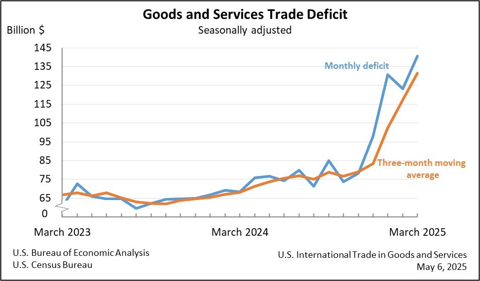
Table IIA-2B provides the US international trade balance, exports and imports of goods and services on an annual basis from 1992 to 2016. The trade balance deteriorated sharply over the long term. The US has a large deficit in goods or exports less imports of goods but it has a surplus in services that helps to reduce the trade account deficit or exports less imports of goods and services. The current account deficit of the US not seasonally adjusted decreased from $115 billion in IQ2016 to $90 billion in IQ2017, increasing to $134 billion in IIQ2017 (https://www.bea.gov/international/index.htm). The current account deficit seasonally adjusted at annual rate increased from 2.3 percent of GDP in IIQ2016 to 2.4 percent of GDP in IQ2017, increasing to 2.6 percent of GDP in IIQ2017 (https://www.bea.gov/international/index.htm https://www.bea.gov/iTable/index_nipa.cfm). The ratio of the current account deficit to GDP has stabilized around 3 percent of GDP compared with much higher percentages before the recession (see Pelaez and Pelaez, The Global Recession Risk (2007), Globalization and the State, Vol. II (2008b), 183-94, Government Intervention in Globalization (2008c), 167-71). The final rows of Table IIA-2B show marginal improvement of the trade deficit from $548,625 million in 2011 to lower $536,773 million in 2012 with exports growing 4.3 percent and imports 3.0 percent. The trade balance improved further to deficit of $461,876 million in 2013 with growth of exports of 3.4 percent while imports virtually stagnated. The trade deficit deteriorated in 2014 to $490,336 million with growth of exports of 3.6 percent and of imports of 4.0 percent. The trade deficit deteriorated in 2015 to $500,445 million with decrease of exports of 4.7 percent and decrease of imports of 3.6 percent. The trade deficit deteriorated in 2016 to $504,793 million with decrease of exports of 2.5 percent and decrease of imports of 1.9 percent. Growth and commodity shocks under alternating inflation waves (https://cmpassocregulationblog.blogspot.com/2017/10/world-inflation-waves-long-term-and.html) have deteriorated the trade deficit from the low of $383,774 million in 2009.
Table IIA-2B, US, International Trade Balance of Goods and Services, Exports and Imports of Goods and Services, SA, Millions of Dollars, Balance of Payments Basis
| Balance | Exports | ∆% | Imports | ∆% | |
| 1960 | 3,508 | 25,940 | NA | 22,432 | NA |
| 1961 | 4,195 | 26,403 | 1.8 | 22,208 | -1.0 |
| 1962 | 3,370 | 27,722 | 5.0 | 24,352 | 9.7 |
| 1963 | 4,210 | 29,620 | 6.8 | 25,410 | 4.3 |
| 1964 | 6,022 | 33,341 | 12.6 | 27,319 | 7.5 |
| 1965 | 4,664 | 35,285 | 5.8 | 30,621 | 12.1 |
| 1966 | 2,939 | 38,926 | 10.3 | 35,987 | 17.5 |
| 1967 | 2,604 | 41,333 | 6.2 | 38,729 | 7.6 |
| 1968 | 250 | 45,543 | 10.2 | 45,293 | 16.9 |
| 1969 | 91 | 49,220 | 8.1 | 49,129 | 8.5 |
| 1970 | 2,254 | 56,640 | 15.1 | 54,386 | 10.7 |
| 1971 | -1,302 | 59,677 | 5.4 | 60,979 | 12.1 |
| 1972 | -5,443 | 67,222 | 12.6 | 72,665 | 19.2 |
| 1973 | 1,900 | 91,242 | 35.7 | 89,342 | 23.0 |
| 1974 | -4,293 | 120,897 | 32.5 | 125,190 | 40.1 |
| 1975 | 12,404 | 132,585 | 9.7 | 120,181 | -4.0 |
| 1976 | -6,082 | 142,716 | 7.6 | 148,798 | 23.8 |
| 1977 | -27,246 | 152,301 | 6.7 | 179,547 | 20.7 |
| 1978 | -29,763 | 178,428 | 17.2 | 208,191 | 16.0 |
| 1979 | -24,565 | 224,131 | 25.6 | 248,696 | 19.5 |
| 1980 | -19,407 | 271,834 | 21.3 | 291,241 | 17.1 |
| 1981 | -16,172 | 294,398 | 8.3 | 310,570 | 6.6 |
| 1982 | -24,156 | 275,236 | -6.5 | 299,391 | -3.6 |
| 1983 | -57,767 | 266,106 | -3.3 | 323,874 | 8.2 |
| 1984 | -109,072 | 291,094 | 9.4 | 400,166 | 23.6 |
| 1985 | -121,880 | 289,070 | -0.7 | 410,950 | 2.7 |
| 1986 | -138,538 | 310,033 | 7.3 | 448,572 | 9.2 |
| 1987 | -151,684 | 348,869 | 12.5 | 500,552 | 11.6 |
| 1988 | -114,566 | 431,149 | 23.6 | 545,715 | 9.0 |
| 1989 | -93,141 | 487,003 | 13.0 | 580,144 | 6.3 |
| 1990 | -80,864 | 535,233 | 9.9 | 616,097 | 6.2 |
| 1991 | -31,135 | 578,344 | 8.1 | 609,479 | -1.1 |
| 1992 | -39,212 | 616,882 | 6.7 | 656,094 | 7.6 |
| 1993 | -70,311 | 642,863 | 4.2 | 713,174 | 8.7 |
| 1994 | -98,493 | 703,254 | 9.4 | 801,747 | 12.4 |
| 1995 | -96,384 | 794,387 | 13.0 | 890,771 | 11.1 |
| 1996 | -104,065 | 851,602 | 7.2 | 955,667 | 7.3 |
| 1997 | -108,273 | 934,453 | 9.7 | 1,042,726 | 9.1 |
| 1998 | -166,140 | 933,174 | -0.1 | 1,099,314 | 5.4 |
| 1999 | -258,617 | 969,867 | 3.9 | 1,228,485 | 11.8 |
| 2000 | -372,517 | 1,075,321 | 10.9 | 1,447,837 | 17.9 |
| 2001 | -361,511 | 1,005,654 | -6.5 | 1,367,165 | -5.6 |
| 2002 | -418,955 | 978,706 | -2.7 | 1,397,660 | 2.2 |
| 2003 | -493,890 | 1,020,418 | 4.3 | 1,514,308 | 8.3 |
| 2004 | -609,883 | 1,161,549 | 13.8 | 1,771,433 | 17.0 |
| 2005 | -714,245 | 1,286,022 | 10.7 | 2,000,267 | 12.9 |
| 2006 | -761,716 | 1,457,642 | 13.3 | 2,219,358 | 11.0 |
| 2007 | -705,375 | 1,653,548 | 13.4 | 2,358,922 | 6.3 |
| 2008 | -708,726 | 1,841,612 | 11.4 | 2,550,339 | 8.1 |
| 2009 | -383,774 | 1,583,053 | -14.0 | 1,966,827 | -22.9 |
| 2010 | -494,658 | 1,853,606 | 17.1 | 2,348,263 | 19.4 |
| 2011 | -548,625 | 2,127,021 | 14.8 | 2,675,646 | 13.9 |
| 2012 | -536,773 | 2,218,989 | 4.3 | 2,755,762 | 3.0 |
| 2013 | -461,876 | 2,293,457 | 3.4 | 2,755,334 | 0.0 |
| 2014 | -490,336 | 2,375,905 | 3.6 | 2,866,241 | 4.0 |
| 2015 | -500,445 | 2,263,907 | -4.7 | 2,764,352 | -3.6 |
| 2016 | -504,793 | 2,208,072 | -2.5 | 2,712,866 | -1.9 |
Source: US Census Bureau
http://www.census.gov/foreign-trade/
Chart IIA-2 of the US Census Bureau provides the US trade account in goods and services SA from Jan 1992 to Sep 2017. There is long-term trend of deterioration of the US trade deficit shown vividly by Chart IIA-2. The global recession from IVQ2007 to IIQ2009 reversed the trend of deterioration. Deterioration resumed together with incomplete recovery and was influenced significantly by the carry trade from zero interest rates to commodity futures exposures (these arguments are elaborated in Pelaez and Pelaez, Financial Regulation after the Global Recession (2009a), 157-66, Regulation of Banks and Finance (2009b), 217-27, International Financial Architecture (2005), 15-18, The Global Recession Risk (2007), 221-5, Globalization and the State Vol. II (2008b), 197-213, Government Intervention in Globalization (2008c), 182-4 http://cmpassocregulationblog.blogspot.com/2011/07/causes-of-2007-creditdollar-crisis.html http://cmpassocregulationblog.blogspot.com/2011/01/professor-mckinnons-bubble-economy.html http://cmpassocregulationblog.blogspot.com/2011/01/world-inflation-quantitative-easing.html http://cmpassocregulationblog.blogspot.com/2011/01/treasury-yields-valuation-of-risk.html http://cmpassocregulationblog.blogspot.com/2010/11/quantitative-easing-theory-evidence-and.html http://cmpassocregulationblog.blogspot.com/2010/12/is-fed-printing-money-what-are.html). Earlier research focused on the long-term external imbalance of the US in the form of trade and current account deficits (Pelaez and Pelaez, The Global Recession Risk (2007), Globalization and the State Vol. II (2008b) 183-94, Government Intervention in Globalization (2008c), 167-71). US external imbalances have not been fully resolved and tend to widen together with improving world economic activity and commodity price shocks. There are additional effects for revaluation of the dollar with the Fed orienting interest rate increases while the European Central Bank and the Bank of Japan determine negative nominal interest rates.
Chart IIA-2, US, Balance of Trade SA, Monthly, Millions of Dollars, Jan 1992-Jul 2017
Source: US Census Bureau
http://www.census.gov/foreign-trade/
Chart IIA-3 of the US Census Bureau provides US exports SA from Jan 1992 to Sep 2017. There was sharp acceleration from 2003 to 2007 during worldwide economic boom and increasing inflation. Exports fell sharply during the financial crisis and global recession from IVQ2007 to IIQ2009. Growth picked up again together with world trade and inflation but stalled in the final segment with less rapid global growth and inflation.
Chart IIA-3, US, Exports SA, Monthly, Millions of Dollars Jan 1992-Jul 2017
Source: US Census Bureau
http://www.census.gov/foreign-trade/
Chart IIA-4 of the US Census Bureau provides US imports SA from Jan 1992 to Sep 2017. Growth was stronger between 2003 and 2007 with worldwide economic boom and inflation. There was sharp drop during the financial crisis and global recession. There is stalling import levels in the final segment resulting from weaker world economic growth and diminishing inflation because of risk aversion and portfolio reallocations from commodity exposures to equities.
Chart IIA-4, US, Imports SA, Monthly, Millions of Dollars Jan 1992-Jul 2017
Source: US Census Bureau
http://www.census.gov/foreign-trade/
There is deterioration of the US trade balance in goods in Table IIA-3 from deficit of $59,435 million in Sep 2016 to deficit of $65,386 million in Sep 2017. The nonpetroleum deficit increased $6878 million while the petroleum deficit decreased $1122 million. Total exports of goods increased 4.7 percent in Sep 2017 relative to a year earlier while total imports increased 6.4 percent. Nonpetroleum exports increased 3.0 percent from Sep 2016 to Sep 2017 while nonpetroleum imports increased 6.1 percent. Petroleum imports increased 11.1 percent.
Table IIA-3, US, International Trade in Goods Balance, Exports and Imports $ Millions and ∆% SA
| Sep 2017 | Sep 2016 | ∆% | |
| Total Balance | -65,386 | -59,435 | |
| Petroleum | -4,008 | -5,130 | |
| Non-Petroleum | -60,104 | -53,226 | |
| Total Exports | 130,581 | 124,741 | 4.7 |
| Petroleum | 10,283 | 7,738 | 32.9 |
| Non-Petroleum | 120,052 | 116,544 | 3.0 |
| Total Imports | 195,967 | 184,175 | 6.4 |
| Petroleum | 14,291 | 12,868 | 11.1 |
| Non-Petroleum | 180,156 | 169,769 | 6.1 |
Details may not add because of rounding and seasonal adjustment
Source: US Census Bureau
http://www.census.gov/foreign-trade/
US exports and imports of goods not seasonally adjusted in Jan-Sep 2017 and Jan-Sep 2016 are in Table IIA-4. The rate of growth of exports was 6.2 percent and 6.4 percent for imports. The US has partial hedge of commodity price increases in exports of agricultural commodities that increased 6.2 percent and of mineral fuels that increased 43.5 percent both because prices of raw materials and commodities increase and fall recurrently because of shocks of risk aversion and portfolio reallocations. The US exports a growing amount of crude oil, increasing 32.4 percent in cumulative Jan-Sep 2017 relative to a year earlier. US exports and imports consist mostly of manufactured products, with less rapidly increasing prices. US manufactured exports increased 3.9 percent while manufactured imports increased 4.8 percent. Significant part of the US trade imbalance originates in imports of mineral fuels increasing 30.5 percent and petroleum increasing 30.5 percent with wide oscillations in oil prices. The limited hedge in exports of agricultural commodities and mineral fuels compared with substantial imports of mineral fuels and crude oil results in waves of deterioration of the terms of trade of the US, or export prices relative to import prices, originating in commodity price increases caused by carry trades from zero interest rates. These waves are similar to those in worldwide inflation.
Table IIA-4, US, Exports and Imports of Goods, Not Seasonally Adjusted Millions of Dollars and %, Census Basis
| Jan-Sep 2017 $ Millions | Jan-Sep 2016 $ Millions | ∆% | |
| Exports | 1,139,043 | 1,072,894 | 6.2 |
| Manufactured | 813,118 | 782,937 | 3.9 |
| Agricultural | 99,102 | 93,351 | 6.2 |
| Mineral Fuels | 95,250 | 66,395 | 43.5 |
| Petroleum | 72,141 | 54,496 | 32.4 |
| Imports | 1,724,236 | 1,620,770 | 6.4 |
| Manufactured | 1,487,178 | 1,419,134 | 4.8 |
| Agricultural | 90,307 | 85,628 | 5.5 |
| Mineral Fuels | 145,026 | 111,163 | 30.5 |
| Petroleum | 134,988 | 103,465 | 30.5 |
Source: US Census Bureau
http://www.census.gov/foreign-trade/
The current account of the US balance of payments is in Table VI-3A for IIQ201 and IIQ2017. The Bureau of Economic Analysis analyzes as follows (https://www.bea.gov/newsreleases/international/transactions/2017/pdf/trans217.pdf):
“The U.S. current-account deficit increased to $123.1 billion (preliminary) in the second quarter of 2017 from $113.5 billion (revised) in the first quarter of 2017, according to statistics released by the Bureau of Economic Analysis (BEA). The deficit increased to 2.6 percent of current-dollar gross domestic product (GDP) from 2.4 percent in the first quarter. The $9.6 billion increase in the current-account deficit reflected a $7.5 billion increase in the deficit on secondary income, a $2.9 billion decrease in the surplus on primary income, and a $0.8 billion increase in the deficit on goods. These changes were partly offset by a $1.6 billion increase in the surplus on services.”
The US has a large deficit in goods or exports less imports of goods but it has a surplus in services that helps to reduce the trade account deficit or exports less imports of goods and services. The current account deficit of the US not seasonally adjusted increased from $114.9 billion in IIQ2016 to $134.0 billion in IIQ2017. The current account deficit seasonally adjusted at annual rate increased from 2.3 percent of GDP in IIQ2016 to 2.4 percent of GDP in IQ2017, increasing to 2.6 percent of GDP in IIQ2017. The ratio of the current account deficit to GDP has stabilized below 3 percent of GDP compared with much higher percentages before the recession but is combined now with much higher imbalance in the Treasury budget (see Pelaez and Pelaez, The Global Recession Risk (2007), Globalization and the State, Vol. II (2008b), 183-94, Government Intervention in Globalization (2008c), 167-71). There is still a major challenge in the combined deficits in current account and in federal budgets.
Table VI-3A, US, Balance of Payments, Millions of Dollars NSA
| IIQ2016 | IIQ2017 | Difference | |
| Goods Balance | -186,924 | -204,290 | -17,366 |
| X Goods | 364,780 | 385,684 | 5.7 ∆% |
| M Goods | -551,704 | -589,974 | 6.9 ∆% |
| Services Balance | 54,508 | 54,111 | 397 |
| X Services | 183,263 | 190,512 | 4.0 ∆% |
| M Services | -128,755 | -136,400 | 5.9 ∆% |
| Balance Goods and Services | -132,416 | -150,179 | -17,763 |
| Exports of Goods and Services and Income Receipts | 786,186 | 834,952 | |
| Imports of Goods and Services and Income Payments | -901,072 | -968,907 | |
| Current Account Balance | -114,886 | -133,954 | -19,068 |
| % GDP | IIQ2016 | IIQ2017 | IQ2017 |
| 2.3 | 2.6 | 2.4 |
X: exports; M: imports
Balance on Current Account = Exports of Goods and Services – Imports of Goods and Services and Income Payments
Source: Bureau of Economic Analysis
http://www.bea.gov/international/index.htm#bop
In their classic work on “unpleasant monetarist arithmetic,” Sargent and Wallace (1981, 2) consider a regime of domination of monetary policy by fiscal policy (emphasis added):
“Imagine that fiscal policy dominates monetary policy. The fiscal authority independently sets its budgets, announcing all current and future deficits and surpluses and thus determining the amount of revenue that must be raised through bond sales and seignorage. Under this second coordination scheme, the monetary authority faces the constraints imposed by the demand for government bonds, for it must try to finance with seignorage any discrepancy between the revenue demanded by the fiscal authority and the amount of bonds that can be sold to the public. Suppose that the demand for government bonds implies an interest rate on bonds greater than the economy’s rate of growth. Then if the fiscal authority runs deficits, the monetary authority is unable to control either the growth rate of the monetary base or inflation forever. If the principal and interest due on these additional bonds are raised by selling still more bonds, so as to continue to hold down the growth of base money, then, because the interest rate on bonds is greater than the economy’s growth rate, the real stock of bonds will growth faster than the size of the economy. This cannot go on forever, since the demand for bonds places an upper limit on the stock of bonds relative to the size of the economy. Once that limit is reached, the principal and interest due on the bonds already sold to fight inflation must be financed, at least in part, by seignorage, requiring the creation of additional base money.”
The alternative fiscal scenario of the CBO (2012NovCDR, 2013Sep17) resembles an economic world in which eventually the placement of debt reaches a limit of what is proportionately desired of US debt in investment portfolios. This unpleasant environment is occurring in various European countries.
The current real value of government debt plus monetary liabilities depends on the expected discounted values of future primary surpluses or difference between tax revenue and government expenditure excluding interest payments (Cochrane 2011Jan, 27, equation (16)). There is a point when adverse expectations about the capacity of the government to generate primary surpluses to honor its obligations can result in increases in interest rates on government debt.
First, Unpleasant Monetarist Arithmetic. Fiscal policy is described by Sargent and Wallace (1981, 3, equation 1) as a time sequence of D(t), t = 1, 2,…t, …, where D is real government expenditures, excluding interest on government debt, less real tax receipts. D(t) is the real deficit excluding real interest payments measured in real time t goods. Monetary policy is described by a time sequence of H(t), t=1,2,…t, …, with H(t) being the stock of base money at time t. In order to simplify analysis, all government debt is considered as being only for one time period, in the form of a one-period bond B(t), issued at time t-1 and maturing at time t. Denote by R(t-1) the real rate of interest on the one-period bond B(t) between t-1 and t. The measurement of B(t-1) is in terms of t-1 goods and [1+R(t-1)] “is measured in time t goods per unit of time t-1 goods” (Sargent and Wallace 1981, 3). Thus, B(t-1)[1+R(t-1)] brings B(t-1) to maturing time t. B(t) represents borrowing by the government from the private sector from t to t+1 in terms of time t goods. The price level at t is denoted by p(t). The budget constraint of Sargent and Wallace (1981, 3, equation 1) is:
D(t) = {[H(t) – H(t-1)]/p(t)} + {B(t) – B(t-1)[1 + R(t-1)]} (1)
Equation (1) states that the government finances its real deficits into two portions. The first portion, {[H(t) – H(t-1)]/p(t)}, is seigniorage, or “printing money.” The second part,
{B(t) – B(t-1)[1 + R(t-1)]}, is borrowing from the public by issue of interest-bearing securities. Denote population at time t by N(t) and growing by assumption at the constant rate of n, such that:
N(t+1) = (1+n)N(t), n>-1 (2)
The per capita form of the budget constraint is obtained by dividing (1) by N(t) and rearranging:
B(t)/N(t) = {[1+R(t-1)]/(1+n)}x[B(t-1)/N(t-1)]+[D(t)/N(t)] – {[H(t)-H(t-1)]/[N(t)p(t)]} (3)
On the basis of the assumptions of equal constant rate of growth of population and real income, n, constant real rate of return on government securities exceeding growth of economic activity and quantity theory equation of demand for base money, Sargent and Wallace (1981) find that “tighter current monetary policy implies higher future inflation” under fiscal policy dominance of monetary policy. That is, the monetary authority does not permanently influence inflation, lowering inflation now with tighter policy but experiencing higher inflation in the future.
Second, Unpleasant Fiscal Arithmetic. The tool of analysis of Cochrane (2011Jan, 27, equation (16)) is the government debt valuation equation:
(Mt + Bt)/Pt = Et∫(1/Rt, t+τ)st+τdτ (4)
Equation (4) expresses the monetary, Mt, and debt, Bt, liabilities of the government, divided by the price level, Pt, in terms of the expected value discounted by the ex-post rate on government debt, Rt, t+τ, of the future primary surpluses st+τ, which are equal to Tt+τ – Gt+τ or difference between taxes, T, and government expenditures, G. Cochrane (2010A) provides the link to a web appendix demonstrating that it is possible to discount by the ex post Rt, t+τ. The second equation of Cochrane (2011Jan, 5) is:
MtV(it, ·) = PtYt (5)
Conventional analysis of monetary policy contends that fiscal authorities simply adjust primary surpluses, s, to sanction the price level determined by the monetary authority through equation (5), which deprives the debt valuation equation (4) of any role in price level determination. The simple explanation is (Cochrane 2011Jan, 5):
“We are here to think about what happens when [4] exerts more force on the price level. This change may happen by force, when debt, deficits and distorting taxes become large so the Treasury is unable or refuses to follow. Then [4] determines the price level; monetary policy must follow the fiscal lead and ‘passively’ adjust M to satisfy [5]. This change may also happen by choice; monetary policies may be deliberately passive, in which case there is nothing for the Treasury to follow and [4] determines the price level.”
An intuitive interpretation by Cochrane (2011Jan 4) is that when the current real value of government debt exceeds expected future surpluses, economic agents unload government debt to purchase private assets and goods, resulting in inflation. If the risk premium on government debt declines, government debt becomes more valuable, causing a deflationary effect. If the risk premium on government debt increases, government debt becomes less valuable, causing an inflationary effect.
There are multiple conclusions by Cochrane (2011Jan) on the debt/dollar crisis and Global recession, among which the following three:
(1) The flight to quality that magnified the recession was not from goods into money but from private-sector securities into government debt because of the risk premium on private-sector securities; monetary policy consisted of providing liquidity in private-sector markets suffering stress
(2) Increases in liquidity by open-market operations with short-term securities have no impact; quantitative easing can affect the timing but not the rate of inflation; and purchase of private debt can reverse part of the flight to quality
(3) The debt valuation equation has a similar role as the expectation shifting the Phillips curve such that a fiscal inflation can generate stagflation effects similar to those occurring from a loss of anchoring expectations.
This analysis suggests that there may be a point of saturation of demand for United States financial liabilities without an increase in interest rates on Treasury securities. A risk premium may develop on US debt. Such premium is not apparent currently because of distressed conditions in the world economy and international financial system. Risk premiums are observed in the spread of bonds of highly indebted countries in Europe relative to bonds of the government of Germany.
The issue of global imbalances centered on the possibility of a disorderly correction (Pelaez and Pelaez, The Global Recession Risk (2007), Globalization and the State Vol. II (2008b) 183-94, Government Intervention in Globalization (2008c), 167-71). Such a correction has not occurred historically but there is no argument proving that it could not occur. The need for a correction would originate in unsustainable large and growing United States current account deficits (CAD) and net international investment position (NIIP) or excess of financial liabilities of the US held by foreigners net relative to financial liabilities of foreigners held by US residents. The IMF estimated that the US could maintain a CAD of two to three percent of GDP without major problems (Rajan 2004). The threat of disorderly correction is summarized by Pelaez and Pelaez, The Global Recession Risk (2007), 15):
“It is possible that foreigners may be unwilling to increase their positions in US financial assets at prevailing interest rates. An exit out of the dollar could cause major devaluation of the dollar. The depreciation of the dollar would cause inflation in the US, leading to increases in American interest rates. There would be an increase in mortgage rates followed by deterioration of real estate values. The IMF has simulated that such an adjustment would cause a decline in the rate of growth of US GDP to 0.5 percent over several years. The decline of demand in the US by four percentage points over several years would result in a world recession because the weakness in Europe and Japan could not compensate for the collapse of American demand. The probability of occurrence of an abrupt adjustment is unknown. However, the adverse effects are quite high, at least hypothetically, to warrant concern.”
The United States could be moving toward a situation typical of heavily indebted countries, requiring fiscal adjustment and increases in productivity to become more competitive internationally. The CAD and NIIP of the United States are not observed in full deterioration because the economy is well below trend. There are two complications in the current environment relative to the concern with disorderly correction in the first half of the past decade. In the release of Jun 14, 2013, the Bureau of Economic Analysis (http://www.bea.gov/newsreleases/international/transactions/2013/pdf/trans113.pdf) informs of revisions of US data on US international transactions since 1999:
“The statistics of the U.S. international transactions accounts released today have been revised for the first quarter of 1999 to the fourth quarter of 2012 to incorporate newly available and revised source data, updated seasonal adjustments, changes in definitions and classifications, and improved estimating methodologies.”
The BEA introduced new concepts and methods (http://www.bea.gov/international/concepts_methods.htm) in comprehensive restructuring on Jun 18, 2014 (http://www.bea.gov/international/modern.htm):
“BEA introduced a new presentation of the International Transactions Accounts on June 18, 2014 and will introduce a new presentation of the International Investment Position on June 30, 2014. These new presentations reflect a comprehensive restructuring of the international accounts that enhances the quality and usefulness of the accounts for customers and bring the accounts into closer alignment with international guidelines.”
Table VI-3B provides data on the US fiscal and balance of payments imbalances incorporating all revisions and methods. In 2007, the federal deficit of the US was $161 billion corresponding to 1.1 percent of GDP while the Congressional Budget Office estimates the federal deficit in 2012 at $1087 billion or 6.8 percent of GDP. The estimate of the deficit for 2013 is $680 billion or 4.1 percent of GDP. The combined record federal deficits of the US from 2009 to 2012 are $5094 billion or 31.6 percent of the estimate of GDP for fiscal year 2012 implicit in the CBO (CBO 2013Sep11) estimate of debt/GDP. The deficits from 2009 to 2012 exceed one trillion dollars per year, adding to $5.094 trillion in four years, using the fiscal year deficit of $1087 billion for fiscal year 2012, which is the worst fiscal performance since World War II. Federal debt in 2007 was $5035 billion, slightly less than the combined deficits from 2009 to 2012 of $5094 billion. Federal debt in 2012 was 70.4 percent of GDP (CBO 2015Jan26) and 72.6 percent of GDP in 2013 (http://www.cbo.gov/). This situation may worsen in the future (CBO 2013Sep17):
“Between 2009 and 2012, the federal government recorded the largest budget deficits relative to the size of the economy since 1946, causing federal debt to soar. Federal debt held by the public is now about 73 percent of the economy’s annual output, or gross domestic product (GDP). That percentage is higher than at any point in U.S. history except a brief period around World War II, and it is twice the percentage at the end of 2007. If current laws generally remained in place, federal debt held by the public would decline slightly relative to GDP over the next several years, CBO projects. After that, however, growing deficits would ultimately push debt back above its current high level. CBO projects that federal debt held by the public would reach 100 percent of GDP in 2038, 25 years from now, even without accounting for the harmful effects that growing debt would have on the economy. Moreover, debt would be on an upward path relative to the size of the economy, a trend that could not be sustained indefinitely.
The gap between federal spending and revenues would widen steadily after 2015 under the assumptions of the extended baseline, CBO projects. By 2038, the deficit would be 6½ percent of GDP, larger than in any year between 1947 and 2008, and federal debt held by the public would reach 100 percent of GDP, more than in any year except 1945 and 1946. With such large deficits, federal debt would be growing faster than GDP, a path that would ultimately be unsustainable.
Incorporating the economic effects of the federal policies that underlie the extended baseline worsens the long-term budget outlook. The increase in debt relative to the size of the economy, combined with an increase in marginal tax rates (the rates that would apply to an additional dollar of income), would reduce output and raise interest rates relative to the benchmark economic projections that CBO used in producing the extended baseline. Those economic differences would lead to lower federal revenues and higher interest payments. With those effects included, debt under the extended baseline would rise to 108 percent of GDP in 2038.”
Table VI-3B, US, Current Account, NIIP, Fiscal Balance, Nominal GDP, Federal Debt and Direct Investment, Dollar Billions and %
| 2007 | 2008 | 2009 | 2010 | 2011 | |
| Goods & | -705 | -709 | -384 | -495 | -549 |
| Primary Income | 85 | 130 | 115 | 168 | 211 |
| Secondary Income | -91 | -102 | -104 | -104 | -107 |
| Current Account | -711 | -681 | -373 | -431 | -445 |
| NGDP | 14478 | 14719 | 14419 | 14964 | 15518 |
| Current Account % GDP | -4.9 | -4.6 | -2.6 | -2.9 | -2.9 |
| NIIP | -1279 | -3995 | -2628 | -2512 | -4455 |
| US Owned Assets Abroad | 20705 | 19423 | 19426 | 21767 | 22209 |
| Foreign Owned Assets in US | 21984 | 23418 | 22054 | 24279 | 26664 |
| NIIP % GDP | -8.8 | -27.1 | -18.2 | -16.8 | -28.7 |
| Exports | 2559 | 2742 | 2283 | 2625 | 2983 |
| NIIP % | -50 | -145 | -115 | -95 | -149 |
| DIA MV | 5858 | 3707 | 4945 | 5486 | 5215 |
| DIUS MV | 4134 | 3091 | 3619 | 4099 | 4199 |
| Fiscal Balance | -161 | -459 | -1413 | -1294 | -1300 |
| Fiscal Balance % GDP | -1.1 | -3.1 | -9.8 | -8.7 | -8.5 |
| Federal Debt | 5035 | 5803 | 7545 | 9019 | 10128 |
| Federal Debt % GDP | 35.2 | 39.3 | 52.3 | 60.9 | 65.9 |
| Federal Outlays | 2729 | 2983 | 3518 | 3457 | 3603 |
| ∆% | 2.8 | 9.3 | 17.9 | -1.7 | 4.2 |
| % GDP | 19.1 | 20.2 | 24.4 | 23.4 | 23.4 |
| Federal Revenue | 2568 | 2524 | 2105 | 2163 | 2303 |
| ∆% | 6.7 | -1.7 | -16.6 | 2.7 | 6.5 |
| % GDP | 17.9 | 17.1 | 14.6 | 14.6 | 15.0 |
| 2012 | 2013 | 2014 | 2015 | 2016 | |
| Goods & | -537 | -462 | -490 | -500 | -505 |
| Primary Income | 207 | 206 | 210 | 181 | 173 |
| Secondary Income | -97 | -94 | -94 | -115 | -120 |
| Current Account | -426 | -350 | -374 | -434 | -452 |
| NGDP | 16155 | 16692 | 17428 | 18121 | 18625 |
| Current Account % GDP | -2.6 | -2.1 | -2.1 | -2.4 | -2.4 |
| NIIP | -4518 | -5373 | -6980 | -7493 | -8318 |
| US Owned Assets Abroad | 22562 | 24145 | 24832 | 23352 | 23849 |
| Foreign Owned Assets in US | 27080 | 29517 | 31813 | 30846 | 32168 |
| NIIP % GDP | -28.0 | -32.2 | -40.1 | -41.3 | -44.7 |
| Exports | 3096 | 3212 | 3333 | 3173 | 3157 |
| NIIP % | -146 | -167 | -209 | -236 | -263 |
| DIA MV | 5969 | 7121 | 7189 | 6999 | 7375 |
| DIUS MV | 4662 | 5815 | 6370 | 6701 | 7569 |
| Fiscal Balance | -1087 | -680 | -485 | -439 | -587 |
| Fiscal Balance % GDP | -6.8 | -4.1 | -2.8 | -2.4 | -3.2 |
| Federal Debt | 11281 | 11983 | 12780 | 13117 | 14168 |
| Federal Debt % GDP | 70.4 | 72.6 | 74.2 | 73.3 | 77.0 |
| Federal Outlays | 3537 | 3455 | 3506 | 3688 | 3853 |
| ∆% | -1.8 | -2.3 | 1.5 | 5.2 | 4.5 |
| % GDP | 22.1 | 20.9 | 20.4 | 20.6 | 20.9 |
| Federal Revenue | 2450 | 2775 | 3022 | 3250 | 3268 |
| ∆% | 6.4 | 13.3 | 8.9 | 7.6 | 0.5 |
| % GDP | 15.3 | 16.8 | 17.5 | 18.2 | 17.8 |
Sources:
Notes: NGDP: nominal GDP or in current dollars; NIIP: Net International Investment Position; DIA MV: US Direct Investment Abroad at Market Value; DIUS MV: Direct Investment in the US at Market Value. There are minor discrepancies in the decimal point of percentages of GDP between the balance of payments data and federal debt, outlays, revenue and deficits in which the original number of the CBO source is maintained. See Bureau of Economic Analysis, US International Economic Accounts: Concepts and Methods. 2014. Washington, DC: BEA, Department of Commerce, Jun 2014 http://www.bea.gov/international/concepts_methods.htm These discrepancies do not alter conclusions. Budget http://www.cbo.gov/
https://www.cbo.gov/about/products/budget-economic-data#6
https://www.cbo.gov/about/products/budget_economic_data#3
https://www.cbo.gov/about/products/budget-economic-data#2
https://www.cbo.gov/about/products/budget_economic_data#2 Balance of Payments and NIIP http://www.bea.gov/international/index.htm#bop Gross Domestic Product, Bureau of Economic Analysis (BEA) http://www.bea.gov/iTable/index_nipa.cfm
The most recent CBO long-term budget on Mar 27, 2017, projects US federal debt at 150.0 percent of GDP in 2047 (Congressional Budget Office, The 2017 Long-term Budget Outlook. Washington, DC, Mar 30, 2017 https://www.cbo.gov/publication/52480).
Table VI-3C provides quarterly estimates NSA of the external imbalance of the United States. The current account deficit seasonally adjusted increases from 2.3 percent of GDP in IIQ2016 to 2.4 percent in IIIQ2016. The current account stabilizes to 2.4 percent of GDP in IVQ2016. The deficit does not change to 2.4 percent in IQ2017 and increases to 2.6 percent in IIQ2017. The absolute value of the net international investment position decreases from minus $8.3 trillion in IIQ2016 to minus $8.0 trillion in IIIQ2016, increasing at minus $8.3 trillion in IVQ2016. The absolute value of the net international investment position decreases to minus $8.1 trillion in IQ2017 and decreases to minus $7.9 trillion in IIQ2017. The BEA explains as follows (https://www.bea.gov/newsreleases/international/intinv/2017/pdf/intinv217.pdf):
“The U.S. net international investment position increased to -$7,934.9 billion (preliminary) at the end of the second quarter of 2017 from -$8,091.6 billion (revised) at the end of the first quarter, according to statistics released today by the Bureau of Economic Analysis (BEA). The $156.7 billion increase reflected a $1,004.2 billion increase in U.S. assets and an $847.5 billion increase in U.S. liabilities.”
The BEA explains further (https://www.bea.gov/newsreleases/international/intinv/2017/pdf/intinv217.pdf): “The $156.7 billion increase reflected net financial transactions of –$107.5 billion and net other changes in position, such as price and exchange-rate changes, of $264.2 billion.
The net investment position increased 1.9 percent in the second quarter, compared with an increase of 2.7 percent in the first quarter, and an average quarterly decrease of 5.6 percent from the first quarter of 2011 through the fourth quarter of 2016.
U.S. assets increased $1,004.2 billion to $25,937.6 billion at the end of the second quarter, mostly reflecting increases in portfolio investment and direct investment assets. Assets excluding financial derivatives increased $1,019.6 billion to $24,006.3 billion. The increase resulted from other changes in position of $657.3 billion and financial transactions of $362.2 billion (table A). Other changes in position mostly reflected the appreciation of major foreign currencies against the U.S. dollar that raised the value of assets in dollar terms. Financial transactions mostly reflected net acquisition of portfolio investment and direct investment equity assets. Liabilities excluding financial derivatives increased $858.3 billion to $31,978.2 billion. The increase resulted from financial transactions of $479.1 billion and other changes in position of $379.2 billion (table A). Financial transactions mostly reflected net incurrence of portfolio investment liabilities. Other changes in position mostly reflected price increases on portfolio investment and direct investment liabilities.”
The net investment position increased 2.1 percent in the first quarter, compared with a decrease of 3.5 percent in the fourth quarter and an average quarterly decrease of 5.7 percent from the first quarter of 2011 through the third quarter of 2016. U.S. assets increased $983.8 billion to $24,833.2 billion at the end of the first quarter. Assets excluding financial derivatives increased $1,246.1 billion to $22,886.5 billion, mostly reflecting increases in portfolio investment and direct investment assets. The $1,246.1 billion increase resulted from other changes in position of $951.9 billion and financial transactions of $294.1 billion (table A). Other changes in position mostly reflected price increases on portfolio investment and direct investment equity assets and the appreciation of major foreign currencies against the U.S. dollar that raised the value of assets in dollar terms. Financial derivatives decreased $262.3 billion to $1,946.7 billion, reflecting decreases in single currency interest rate contracts and foreign exchange contracts. U.S. liabilities increased $806.6 billion to $32,974.5 billion at the end of the first quarter. Liabilities excluding financial derivatives increased $1,049.2 billion to $31,069.4 billion, mostly reflecting increases in portfolio investment and direct investment liabilities. The $1,049.2 billion increase resulted from other changes in position of $656.1 billion and financial transactions of $393.2 billion (table A). Other changes in position were driven by price increases on portfolio investment and direct investment equity liabilities. Financial derivatives decreased $242.6 billion to $1,905.1 billion, reflecting decreases in single currency interest rate contracts and foreign exchange contracts.”
Table VI-3C, US, Current Account, NIIP, Fiscal Balance, Nominal GDP, Federal Debt and Direct Investment, Dollar Billions and % NSA
| IIQ2016 | IIIQ2016 | IVQ2016 | IQ2017 | IIQ2017 | |
| Goods & | -132 | -136 | -132 | -113 | -150 |
| Primary Income | 43 | 43 | 51 | 49 | 47 |
| Secondary Income | -26 | -32 | -31 | -26 | -31 |
| Current Account | -115 | -126 | -112 | -90 | -134 |
| Current Account % GDP | -2.3 | -2.4 | -2.4 | -2.4 | -2.6 |
| NIIP | -8292 | -8036 | -8318 | -8092 | -7935 |
| US Owned Assets Abroad | 24558 | 24839 | 23849 | 24933 | 25938 |
| Foreign Owned Assets in US | -32851 | -32875 | -32168 | -33025 | -33873 |
| DIA MV | 7002 | 7392 | 7375 | 7895 | 8202 |
| DIA MV Equity | 5780 | 6147 | 6172 | 6609 | 6918 |
| DIUS MV | 7123 | 7424 | 7569 | 7952 | 8162 |
| DIUS MV Equity | 5377 | 5607 | 5784 | 6153 | 6353 |
Notes: NIIP: Net International Investment Position; DIA MV: US Direct Investment Abroad at Market Value; DIUS MV: Direct Investment in the US at Market Value. See Bureau of Economic Analysis, US International Economic Accounts: Concepts and Methods. 2014. Washington, DC: BEA, Department of Commerce, Jun 2014 http://www.bea.gov/international/concepts_methods.htm
Chart VI-3C of the US Bureau of Economic Analysis provides the quarterly and annual US net international investment position (NIIP) NSA in billion dollars. The NIIP deteriorated in 2008, improving in 2009-2011 followed by deterioration after 2012.
Chart VI-3C, US Net International Investment Position, NSA, Billion US Dollars
Source: Bureau of Economic Analysis
http://www.bea.gov/newsreleases/international/intinv/intinvnewsrelease.htm
Chart VI-10 of the Board of Governors of the Federal Reserve System provides the overnight Fed funds rate on business days from Jul 1, 1954 at 1.13 percent through Jan 10, 1979, at 9.91 percent per year, to Nov 9, 2017, at 1.16 percent per year. US recessions are in shaded areas according to the reference dates of the NBER (http://www.nber.org/cycles.html). In the Fed effort to control the “Great Inflation” of the 1970s (http://cmpassocregulationblog.blogspot.com/2011/05/slowing-growth-global-inflation-great.html http://cmpassocregulationblog.blogspot.com/2011/04/new-economics-of-rose-garden-turned.html http://cmpassocregulationblog.blogspot.com/2011/03/is-there-second-act-of-us-great.html and Appendix I The Great Inflation; see Taylor 1993, 1997, 1998LB, 1999, 2012FP, 2012Mar27, 2012Mar28, 2012JMCB and http://cmpassocregulationblog.blogspot.com/2017/01/rules-versus-discretionary-authorities.html http://cmpassocregulationblog.blogspot.com/2012/06/rules-versus-discretionary-authorities.html), the fed funds rate increased from 8.34 percent on Jan 3, 1979 to a high in Chart VI-10 of 22.36 percent per year on Jul 22, 1981 with collateral adverse effects in the form of impaired savings and loans associations in the United States, emerging market debt and money-center banks (see Pelaez and Pelaez, Regulation of Banks and Finance (2009b), 72-7; Pelaez 1986, 1987). Another episode in Chart VI-10 is the increase in the fed funds rate from 3.15 percent on Jan 3, 1994, to 6.56 percent on Dec 21, 1994, which also had collateral effects in impairing emerging market debt in Mexico and Argentina and bank balance sheets in a world bust of fixed income markets during pursuit by central banks of non-existing inflation (Pelaez and Pelaez, International Financial Architecture (2005), 113-5). Another interesting policy impulse is the reduction of the fed funds rate from 7.03 percent on Jul 3, 2000, to 1.00 percent on Jun 22, 2004, in pursuit of equally non-existing deflation (Pelaez and Pelaez, International Financial Architecture (2005), 18-28, The Global Recession Risk (2007), 83-85), followed by increments of 25 basis points from Jun 2004 to Jun 2006, raising the fed funds rate to 5.25 percent on Jul 3, 2006 in Chart VI-10. Central bank commitment to maintain the fed funds rate at 1.00 percent induced adjustable-rate mortgages (ARMS) linked to the fed funds rate. Lowering the interest rate near the zero bound in 2003-2004 caused the illusion of permanent increases in wealth or net worth in the balance sheets of borrowers and also of lending institutions, securitized banking and every financial institution and investor in the world. The discipline of calculating risks and returns was seriously impaired. The objective of monetary policy was to encourage borrowing, consumption and investment but the exaggerated stimulus resulted in a financial crisis of major proportions as the securitization that had worked for a long period was shocked with policy-induced excessive risk, imprudent credit, high leverage and low liquidity by the incentive to finance everything overnight at interest rates close to zero, from adjustable rate mortgages (ARMS) to asset-backed commercial paper of structured investment vehicles (SIV).
The consequences of inflating liquidity and net worth of borrowers were a global hunt for yields to protect own investments and money under management from the zero interest rates and unattractive long-term yields of Treasuries and other securities. Monetary policy distorted the calculations of risks and returns by households, business and government by providing central bank cheap money. Short-term zero interest rates encourage financing of everything with short-dated funds, explaining the SIVs created off-balance sheet to issue short-term commercial paper with the objective of purchasing default-prone mortgages that were financed in overnight or short-dated sale and repurchase agreements (Pelaez and Pelaez, Financial Regulation after the Global Recession, 50-1, Regulation of Banks and Finance, 59-60, Globalization and the State Vol. I, 89-92, Globalization and the State Vol. II, 198-9, Government Intervention in Globalization, 62-3, International Financial Architecture, 144-9). ARMS were created to lower monthly mortgage payments by benefitting from lower short-dated reference rates. Financial institutions economized in liquidity that was penalized with near zero interest rates. There was no perception of risk because the monetary authority guaranteed a minimum or floor price of all assets by maintaining low interest rates forever or equivalent to writing an illusory put option on wealth. Subprime mortgages were part of the put on wealth by an illusory put on house prices. The housing subsidy of $221 billion per year created the impression of ever-increasing house prices. The suspension of auctions of 30-year Treasuries was designed to increase demand for mortgage-backed securities, lowering their yield, which was equivalent to lowering the costs of housing finance and refinancing. Fannie and Freddie purchased or guaranteed $1.6 trillion of nonprime mortgages and worked with leverage of 75:1 under Congress-provided charters and lax oversight. The combination of these policies resulted in high risks because of the put option on wealth by near zero interest rates, excessive leverage because of cheap rates, low liquidity because of the penalty in the form of low interest rates and unsound credit decisions because the put option on wealth by monetary policy created the illusion that nothing could ever go wrong, causing the credit/dollar crisis and global recession (Pelaez and Pelaez, Financial Regulation after the Global Recession, 157-66, Regulation of Banks, and Finance, 217-27, International Financial Architecture, 15-18, The Global Recession Risk, 221-5, Globalization and the State Vol. II, 197-213, Government Intervention in Globalization, 182-4). A final episode in Chart VI-10 is the reduction of the fed funds rate from 5.41 percent on Aug 9, 2007, to 2.97 percent on October 7, 2008, to 0.12 percent on Dec 5, 2008 and close to zero throughout a long period with the final point at 1.16 percent on Nov 9, 2017. Evidently, this behavior of policy would not have occurred had there been theory, measurements and forecasts to avoid these violent oscillations that are clearly detrimental to economic growth and prosperity without inflation. The Chair of the Board of Governors of the Federal Reserve System, Janet L. Yellen, stated on Jul 10, 2015 that (http://www.federalreserve.gov/newsevents/speech/yellen20150710a.htm):
“Based on my outlook, I expect that it will be appropriate at some point later this year to take the first step to raise the federal funds rate and thus begin normalizing monetary policy. But I want to emphasize that the course of the economy and inflation remains highly uncertain, and unanticipated developments could delay or accelerate this first step. I currently anticipate that the appropriate pace of normalization will be gradual, and that monetary policy will need to be highly supportive of economic activity for quite some time. The projections of most of my FOMC colleagues indicate that they have similar expectations for the likely path of the federal funds rate. But, again, both the course of the economy and inflation are uncertain. If progress toward our employment and inflation goals is more rapid than expected, it may be appropriate to remove monetary policy accommodation more quickly. However, if progress toward our goals is slower than anticipated, then the Committee may move more slowly in normalizing policy.”
There is essentially the same view in the Testimony of Chair Yellen in delivering the Semiannual Monetary Policy Report to the Congress on Jul 15, 2015 (http://www.federalreserve.gov/newsevents/testimony/yellen20150715a.htm). The FOMC (Federal Open Market Committee) raised the fed funds rate to ¼ to ½ percent at its meeting on Dec 16, 2015 (http://www.federalreserve.gov/newsevents/press/monetary/20151216a.htm).
It is a forecast mandate because of the lags in effect of monetary policy impulses on income and prices (Romer and Romer 2004). The intention is to reduce unemployment close to the “natural rate” (Friedman 1968, Phelps 1968) of around 5 percent and inflation at or below 2.0 percent. If forecasts were reasonably accurate, there would not be policy errors. A commonly analyzed risk of zero interest rates is the occurrence of unintended inflation that could precipitate an increase in interest rates similar to the Himalayan rise of the fed funds rate from 9.91 percent on Jan 10, 1979, at the beginning in Chart VI-10, to 22.36 percent on Jul 22, 1981. There is a less commonly analyzed risk of the development of a risk premium on Treasury securities because of the unsustainable Treasury deficit/debt of the United States (https://cmpassocregulationblog.blogspot.com/2017/04/mediocre-cyclical-economic-growth-with.html and earlier http://cmpassocregulationblog.blogspot.com/2017/01/twenty-four-million-unemployed-or.html and earlier and earlier http://cmpassocregulationblog.blogspot.com/2016/12/rising-yields-and-dollar-revaluation.html http://cmpassocregulationblog.blogspot.com/2016/07/unresolved-us-balance-of-payments.html and earlier http://cmpassocregulationblog.blogspot.com/2016/04/proceeding-cautiously-in-reducing.html and earlier http://cmpassocregulationblog.blogspot.com/2016/01/weakening-equities-and-dollar.html and earlier http://cmpassocregulationblog.blogspot.com/2015/09/monetary-policy-designed-on-measurable.html and earlier http://cmpassocregulationblog.blogspot.com/2015/06/fluctuating-financial-asset-valuations.html and earlier (http://cmpassocregulationblog.blogspot.com/2015/03/irrational-exuberance-mediocre-cyclical.html and earlier http://cmpassocregulationblog.blogspot.com/2014/12/patience-on-interest-rate-increases.html
and earlier http://cmpassocregulationblog.blogspot.com/2014/09/world-inflation-waves-squeeze-of.html and earlier (http://cmpassocregulationblog.blogspot.com/2014/02/theory-and-reality-of-cyclical-slow.html and earlier (http://cmpassocregulationblog.blogspot.com/2013/02/united-states-unsustainable-fiscal.html). There is not a fiscal cliff or debt limit issue ahead but rather free fall into a fiscal abyss. The combination of the fiscal abyss with zero interest rates could trigger the risk premium on Treasury debt or Himalayan hike in interest rates.
Chart VI-10, US, Fed Funds Rate, Business Days, Jul 1, 1954 to Nov 2, 2017, Percent per Year
Source: Board of Governors of the Federal Reserve System
https://www.federalreserve.gov/datadownload/Choose.aspx?rel=H15
There is a false impression of the existence of a monetary policy “science,” measurements and forecasting with which to steer the economy into “prosperity without inflation.” Market participants are remembering the Great Bond Crash of 1994 shown in Table VI-7G when monetary policy pursued nonexistent inflation, causing trillions of dollars of losses in fixed income worldwide while increasing the fed funds rate from 3 percent in Jan 1994 to 6 percent in Dec. The exercise in Table VI-7G shows a drop of the price of the 30-year bond by 18.1 percent and of the 10-year bond by 14.1 percent. CPI inflation remained almost the same and there is no valid counterfactual that inflation would have been higher without monetary policy tightening because of the long lag in effect of monetary policy on inflation (see Culbertson 1960, 1961, Friedman 1961, Batini and Nelson 2002, Romer and Romer 2004). The pursuit of nonexistent deflation during the past ten years has resulted in the largest monetary policy accommodation in history that created the 2007 financial market crash and global recession and is currently preventing smoother recovery while creating another financial crash in the future. The issue is not whether there should be a central bank and monetary policy but rather whether policy accommodation in doses from zero interest rates to trillions of dollars in the fed balance sheet endangers economic stability.
Table VI-7G, Fed Funds Rates, Thirty and Ten Year Treasury Yields and Prices, 30-Year Mortgage Rates and 12-month CPI Inflation 1994
| 1994 | FF | 30Y | 30P | 10Y | 10P | MOR | CPI |
| Jan | 3.00 | 6.29 | 100 | 5.75 | 100 | 7.06 | 2.52 |
| Feb | 3.25 | 6.49 | 97.37 | 5.97 | 98.36 | 7.15 | 2.51 |
| Mar | 3.50 | 6.91 | 92.19 | 6.48 | 94.69 | 7.68 | 2.51 |
| Apr | 3.75 | 7.27 | 88.10 | 6.97 | 91.32 | 8.32 | 2.36 |
| May | 4.25 | 7.41 | 86.59 | 7.18 | 88.93 | 8.60 | 2.29 |
| Jun | 4.25 | 7.40 | 86.69 | 7.10 | 90.45 | 8.40 | 2.49 |
| Jul | 4.25 | 7.58 | 84.81 | 7.30 | 89.14 | 8.61 | 2.77 |
| Aug | 4.75 | 7.49 | 85.74 | 7.24 | 89.53 | 8.51 | 2.69 |
| Sep | 4.75 | 7.71 | 83.49 | 7.46 | 88.10 | 8.64 | 2.96 |
| Oct | 4.75 | 7.94 | 81.23 | 7.74 | 86.33 | 8.93 | 2.61 |
| Nov | 5.50 | 8.08 | 79.90 | 7.96 | 84.96 | 9.17 | 2.67 |
| Dec | 6.00 | 7.87 | 81.91 | 7.81 | 85.89 | 9.20 | 2.67 |
Notes: FF: fed funds rate; 30Y: yield of 30-year Treasury; 30P: price of 30-year Treasury assuming coupon equal to 6.29 percent and maturity in exactly 30 years; 10Y: yield of 10-year Treasury; 10P: price of 10-year Treasury assuming coupon equal to 5.75 percent and maturity in exactly 10 years; MOR: 30-year mortgage; CPI: percent change of CPI in 12 months
Sources: yields and mortgage rates http://www.federalreserve.gov/releases/h15/data.htm CPI ftp://ftp.bls.gov/pub/special.requests/cpi/cpiai.t
Chart VI-14 provides the overnight fed funds rate, the yield of the 10-year Treasury constant maturity bond, the yield of the 30-year constant maturity bond and the conventional mortgage rate from Jan 1991 to Dec 1996. In Jan 1991, the fed funds rate was 6.91 percent, the 10-year Treasury yield 8.09 percent, the 30-year Treasury yield 8.27 percent and the conventional mortgage rate 9.64 percent. Before monetary policy tightening in Oct 1993, the rates and yields were 2.99 percent for the fed funds, 5.33 percent for the 10-year Treasury, 5.94 for the 30-year Treasury and 6.83 percent for the conventional mortgage rate. After tightening in Nov 1994, the rates and yields were 5.29 percent for the fed funds rate, 7.96 percent for the 10-year Treasury, 8.08 percent for the 30-year Treasury and 9.17 percent for the conventional mortgage rate.
Chart VI-14, US, Overnight Fed Funds Rate, 10-Year Treasury Constant Maturity, 30-Year Treasury Constant Maturity and Conventional Mortgage Rate, Monthly, Jan 1991 to Dec 1996
Source: Board of Governors of the Federal Reserve System
http://www.federalreserve.gov/releases/h15/update/
Chart VI-15 of the Bureau of Labor Statistics provides the all items consumer price index from Jan 1991 to Dec 1996. There does not appear acceleration of consumer prices requiring aggressive tightening.
Chart VI-15, US, Consumer Price Index All Items, Jan 1991 to Dec 1996
Source: Bureau of Labor Statistics
http://www.bls.gov/cpi/data.htm
Chart IV-16 of the Bureau of Labor Statistics provides 12-month percentage changes of the all items consumer price index from Jan 1991 to Dec 1996. Inflation collapsed during the recession from Jul 1990 (III) and Mar 1991 (I) and the end of the Kuwait War on Feb 25, 1991 that stabilized world oil markets. CPI inflation remained almost the same and there is no valid counterfactual that inflation would have been higher without monetary policy tightening because of the long lag in effect of monetary policy on inflation (see Culbertson 1960, 1961, Friedman 1961, Batini and Nelson 2002, Romer and Romer 2004). Policy tightening had adverse collateral effects in the form of emerging market crises in Mexico and Argentina and fixed income markets worldwide.
Chart VI-16, US, Consumer Price Index All Items, Twelve-Month Percentage Change, Jan 1991 to Dec 1996
Source: Bureau of Labor Statistics
http://www.bls.gov/cpi/data.htm
The Congressional Budget Office (CBO 2017Jun29, CBO 2017Jan24) estimates potential GDP, potential labor force and potential labor productivity provided in Table IB-3. The CBO estimates average rate of growth of potential GDP from 1950 to 2016 at 3.2 percent per year. The projected path is significantly lower at 1.8 percent per year from 2017 to 2027. The legacy of the economic cycle expansion from IIIQ2009 to IIQ2017 at 2.2 percent on average is in contrast with 4.0 percent on average in the expansion from IQ1983 to IVQ1990 (https://cmpassocregulationblog.blogspot.com/2017/10/destruction-of-household-nonfinancial.html and earlier https://cmpassocregulationblog.blogspot.com/2017/09/mediocre-cyclical-united-states.html). Subpar economic growth may perpetuate unemployment and underemployment estimated at 21.1 million or 12.5 percent of the effective labor force in Sep 2017 (https://cmpassocregulationblog.blogspot.com/2017/10/twenty-one-million-unemployed-or.html and earlier https://cmpassocregulationblog.blogspot.com/2017/09/twenty-two-million-unemployed-or.html) with much lower hiring than in the period before the current cycle (Section I and earlier (https://cmpassocregulationblog.blogspot.com/2017/09/dollar-devaluation-world-inflation.html).
Table IB-3, US, Congressional Budget Office History and Projections of Potential GDP of US Overall Economy, ∆%
| Potential GDP | Potential Labor Force | Potential Labor Productivity* | |
| Average Annual ∆% | |||
| 1950-1973 | 4.0 | 1.6 | 2.4 |
| 1974-1981 | 3.2 | 2.5 | 0.6 |
| 1982-1990 | 3.4 | 1.7 | 1.7 |
| 1991-2001 | 3.3 | 1.2 | 2.0 |
| 2002-2007 | 2.4 | 1.0 | 1.4 |
| 2008-2016 | 1.4 | 0.5 | 0.9 |
| Total 1950-2016 | 3.2 | 1.4 | 1.7 |
| Projected Average Annual ∆% | |||
| 2017-2020 | 1.7 | 0.5 | 1.2 |
| 2021-2027 | 1.9 | 0.5 | 1.4 |
| 2017-2027 | 1.8 | 0.5 | 1.3 |
*Ratio of potential GDP to potential labor force
Source: CBO, The budget and economic outlook: 2017-2027. Washington, DC, Jan 24, 2017 https://www.cbo.gov/publication/52370 CBO (2014BEOFeb4), CBO, Key assumptions in projecting potential GDP—February 2014 baseline. Washington, DC, Congressional Budget Office, Feb 4, 2014. CBO, The budget and economic outlook: 2015 to 2025. Washington, DC, Congressional Budget Office, Jan 26, 2015. Aug 2016
https://www.cbo.gov/about/products/budget-economic-data#6
Chart IB1-A1 of the Congressional Budget Office provides historical and projected annual growth of United States potential GDP. There is sharp decline of growth of United States potential GDP.
Chart IB-1A1, Congressional Budget Office, Projections of Annual Growth of United States Potential GDP
Source: CBO, The budget and economic outlook: 2017-2027. Washington, DC, Jan 24, 2017 https://www.cbo.gov/publication/52370
https://www.cbo.gov/about/products/budget-economic-data#6
Chart IB-1A of the Congressional Budget Office provides historical and projected potential and actual US GDP. The gap between actual and potential output closes by 2017. Potential output expands at a lower rate than historically. Growth is even weaker relative to trend.
Chart IB-1A, Congressional Budget Office, Estimate of Potential GDP and Gap
Source: Congressional Budget Office
https://www.cbo.gov/publication/49890
Chart IB-1 of the Congressional Budget Office (CBO 2013BEOFeb5) provides actual and potential GDP of the United States from 2000 to 2011 and projected to 2024. Lucas (2011May) estimates trend of United States real GDP of 3.0 percent from 1870 to 2010 and 2.2 percent for per capita GDP. The United States successfully returned to trend growth of GDP by higher rates of growth during cyclical expansion as analyzed by Bordo (2012Sep27, 2012Oct21) and Bordo and Haubrich (2012DR). Growth in expansions following deeper contractions and financial crises was much higher in agreement with the plucking model of Friedman (1964, 1988). The unusual weakness of growth at 2.2 percent on average from IIIQ2009 to IIQ2017 during the current economic expansion in contrast with 4.0 percent on average in the cyclical expansion from IQ1983 to IVQ1990 (https://cmpassocregulationblog.blogspot.com/2017/10/destruction-of-household-nonfinancial.html and earlier https://cmpassocregulationblog.blogspot.com/2017/09/mediocre-cyclical-united-states.html) cannot be explained by the contraction of 4.2 percent of GDP from IVQ2007 to IIQ2009 and the financial crisis. Weakness of growth in the expansion is perpetuating unemployment and underemployment of 21.1 million or 12.5 percent of the labor force as estimated for Sep 2017 (https://cmpassocregulationblog.blogspot.com/2017/10/twenty-one-million-unemployed-or.html and earlier https://cmpassocregulationblog.blogspot.com/2017/09/twenty-two-million-unemployed-or.html). There is no exit from unemployment/underemployment and stagnating real wages because of the collapse of hiring (Section I and earlier (https://cmpassocregulationblog.blogspot.com/2017/09/dollar-devaluation-world-inflation.html). The US economy and labor markets collapsed without recovery. Abrupt collapse of economic conditions can be explained only with cyclic factors (Lazear and Spletzer 2012Jul22) and not by secular stagnation (Hansen 1938, 1939, 1941 with early dissent by Simons 1942).
Chart IB-1, US, Congressional Budget Office, Actual and Projections of Potential GDP, 2000-2024, Trillions of Dollars
Source: Congressional Budget Office, CBO (2013BEOFeb5). The last year in common in both projections is 2017. The revision lowers potential output in 2017 by 7.3 percent relative to the projection in 2007.
Chart IB-2 provides differences in the projections of potential output by the CBO in 2007 and more recently on Feb 4, 2014, which the CBO explains in CBO (2014Feb28).
Chart IB-2, Congressional Budget Office, Revisions of Potential GDP
Source: Congressional Budget Office, 2014Feb 28. Revisions to CBO’s Projection of Potential Output since 2007. Washington, DC, CBO, Feb 28, 2014.
Chart IB-3 provides actual and projected potential GDP from 2000 to 2024. The gap between actual and potential GDP disappears at the end of 2017 (CBO2014Feb4). GDP increases in the projection at 2.5 percent per year.
Chart IB-3, Congressional Budget Office, GDP and Potential GDP
Source: CBO (2013BEOFeb5), CBO, Key assumptions in projecting potential GDP—February 2014 baseline. Washington, DC, Congressional Budget Office, Feb 4, 2014.
Chart IIA2-3 of the Bureau of Economic Analysis of the Department of Commerce shows on the lower negative panel the sharp increase in the deficit in goods and the deficits in goods and services from 1960 to 2012. The upper panel shows the increase in the surplus in services that was insufficient to contain the increase of the deficit in goods and services. The adjustment during the global recession has been in the form of contraction of economic activity that reduced demand for goods.
Chart IIA2-3, US, Balance of Goods, Balance on Services and Balance on Goods and Services, 1960-2013, Millions of Dollars
Source: Bureau of Economic Analysis http://www.bea.gov/iTable/index_ita.cfm
Chart IIA2-4 of the Bureau of Economic Analysis shows exports and imports of goods and services from 1960 to 2012. Exports of goods and services in the upper positive panel have been quite dynamic but have not compensated for the sharp increase in imports of goods. The US economy apparently has become less competitive in goods than in services.
Chart IIA2-4, US, Exports and Imports of Goods and Services, 1960-2013, Millions of Dollars
Source: Bureau of Economic Analysis http://www.bea.gov/iTable/index_ita.cfm
Chart IIA2-5 of the Bureau of Economic Analysis shows the US balance on current account from 1960 to 2012. The sharp devaluation of the dollar resulting from unconventional monetary policy of zero interest rates and elimination of auctions of 30-year Treasury bonds did not adjust the US balance of payments. Adjustment only occurred after the contraction of economic activity during the global recession.
Chart IIA2-5, US, Balance on Current Account, 1960-2013, Millions of Dollars
Source: Bureau of Economic Analysis http://www.bea.gov/iTable/index_ita.cfm
Chart IIA2-6 of the Bureau of Economic Analysis provides real GDP in the US from 1960 to 2016. The contraction of economic activity during the global recession was a major factor in the reduction of the current account deficit as percent of GDP.
Chart IIA2-6, US, Real GDP, 1960-2016, Billions of Chained 2009 Dollars
Source: Bureau of Economic Analysis
http://www.bea.gov/iTable/index_nipa.cfm
Chart IIA2-6, US, Real GDP, 1960-2016, Billions of Chained 2009 Dollars
Source: Bureau of Economic Analysis
http://www.bea.gov/iTable/index_nipa.cfm
Chart IIA-7 provides the US current account deficit on a quarterly basis from 1980 to IQ1983. The deficit is at a lower level because of growth below potential not only in the US but worldwide. The combination of high government debt and deficit with external imbalance restricts potential prosperity in the US.
Chart IIA-7, US, Balance on Current Account, Quarterly, 1980-2013
Source: Bureau of Economic Analysis
http://www.bea.gov/iTable/index_nipa.cfm
Risk aversion channels funds toward US long-term and short-term securities that finance the US balance of payments and fiscal deficits benefitting from risk flight to US dollar denominated assets. There are now temporary interruptions because of fear of rising interest rates that erode prices of US government securities because of mixed signals on monetary policy and exit from the Fed balance sheet of four trillion dollars of securities held outright. Net foreign purchases of US long-term securities (row C in Table VA-4) strengthened from minus $43.2 billion in Jul 2017 to $51.1 billion in Aug
2017. Foreign residents’ purchases minus sales of US long-term securities (row A in Table VA-4) in Jul 2017 of $5.1 billion strengthened to $34.6 billion in Aug 2017. Net US (residents) purchases of long-term foreign securities (row B in Table VA-4) strengthened from minus $3.8 billion in Jun 2017 to $32.6 billion in Aug 2017. Other transactions (row C2 in Table VA-4) changed from minus $44.5 billion in Jul 2017 to minus $16.1 billion in Aug 2017. In Aug 2017,
C = A + B + C2 = $34.6 billion + $32.6 billion - $16.1 billion = $51.1 billion
There are minor rounding errors. There is strengthening demand in Table VA-4 in Aug 2017 in A1 private purchases by residents overseas of US long-term securities of $35.6 billion of which weakening in A11 Treasury securities of $13.7 billion, strengthening in A12 of $9.4 billion in agency securities, strengthening of
$16.7 billion of corporate bonds and weakening of minus $4.2 billion in equities. Worldwide risk aversion causes flight into US Treasury obligations with significant oscillations. Official purchases of securities in row A2 decreased $1.0 billion with decrease of Treasury securities of $2.2 billion in Aug 2017. Official purchases of agency securities decreased $0.2 billion in Aug 2017. Row D shows decrease in Aug 2017 of $34.9 billion in purchases of short-term dollar denominated obligations. Foreign private holdings of US Treasury bills increased $0.7 billion (row D11) with foreign official holdings decreasing $6.5 billion while the category “other” decreased $29.1 billion. Foreign private holdings of US Treasury bills increased $0.7 billion in what could be arbitrage of duration exposures and international risks. Risk aversion of default losses in foreign securities dominates decisions to accept zero interest rates in Treasury securities with no perception of principal losses. In the case of long-term securities, investors prefer to sacrifice inflation and possible duration risk to avoid principal losses with significant oscillations in risk perceptions.
Table VA-1, Net Cross-Borders Flows of US Long-Term Securities, Billion Dollars, NSA
| Aug 2016 12 Months | Aug 2017 12 Months | Jul 2017 | Aug 2017 | |
| A Foreign Purchases less Sales of | 76.1 | 211.1 | 5.1 | 34.6 |
| A1 Private | 401.1 | 372.3 | 18.6 | 35.6 |
| A11 Treasury | 135.5 | 96.5 | 16.2 | 13.7 |
| A12 Agency | 192.5 | 129.5 | 6.7 | 9.4 |
| A13 Corporate Bonds | 150.6 | 99.2 | 3.0 | 16.7 |
| A14 Equities | -77.4 | 47.1 | -7.3 | -4.2 |
| A2 Official | -324.9 | -161.2 | -13.5 | -1.0 |
| A21 Treasury | -340.4 | -194.4 | -16.7 | -2.2 |
| A22 Agency | 29.7 | 32.3 | 3.6 | -0.2 |
| A23 Corporate Bonds | -6.2 | -2.2 | 0.0 | 2.5 |
| A24 Equities | -8.0 | 3.1 | -0.3 | -1.2 |
| B Net US Purchases of LT Foreign Securities | 197.8 | 142.1 | -3.8 | 32.6 |
| B1 Foreign Bonds | 258.2 | 237.9 | 11.7 | 32.2 |
| B2 Foreign Equities | -60.4 | -95.8 | -15.5 | 0.3 |
| C1 Net Transactions | 273.9 | 353.2 | 1.2 | 67.2 |
| C2 Other | -230.7 | -270.9 | -44.5 | -16.1 |
| C Net Foreign Purchases of US LT Securities | 43.2 | 82.4 | -43.2 | 51.1 |
| D Increase in Foreign Holdings of Dollar Denominated Short-term | ||||
| US Securities & Other Liab | 50.3 | 44.2 | 7.4 | -34.9 |
| D1 US Treasury Bills | -12.4 | 6.5 | 3.1 | -5.8 |
| D11 Private | 70.5 | -44.8 | 3.0 | 0.7 |
| D12 Official | -82.9 | 51.3 | 0.1 | -6.5 |
| D2 Other | 62.7 | 37.7 | 4.3 | -29.1 |
C1 = A + B; C = C1+C2
A = A1 + A2
A1 = A11 + A12 + A13 + A14
A2 = A21 + A22 + A23 + A24
B = B1 + B2
D = D1 + D2
Sources: United States Treasury
https://www.treasury.gov/resource-center/data-chart-center/tic/Pages/ticpress.aspx
http://www.treasury.gov/press-center/press-releases/Pages/jl2609.aspx
Table VA-5 provides major foreign holders of US Treasury securities. China is the largest holder with $1200.5 billion in Aug 2017, increasing 3.0 percent from $1166.0 billion in Jul 2017 while increasing $15.4 billion from Aug 2016 or 1.3 percent. The United States Treasury estimates US government debt held by private investors at $11,533 billion in Jun 2017. China’s holding of US Treasury securities represents 10.4 percent of US government marketable interest-bearing debt held by private investors (http://www.fms.treas.gov/bulletin/index.html). Min Zeng, writing on “China plays a big role as US Treasury yields fall,” on Jul 16, 2014, published in the Wall Street Journal (http://online.wsj.com/articles/china-plays-a-big-role-as-u-s-treasury-yields-fall-1405545034?tesla=y&mg=reno64-wsj), finds that acceleration in purchases of US Treasury securities by China has been an important factor in the decline of Treasury yields in 2014. Japan decreased its holdings from $1144.0 billion in Aug 2016 to $1101.7 billion in Aug 2017 or 3.7 percent. The combined holdings of China and Japan in Aug 2017 add to $2302.2 billion, which is equivalent to 20.0 percent of US government marketable interest-bearing securities held by investors of $11,533 billion in Jun 2017 (http://www.fms.treas.gov/bulletin/index.html). Total foreign holdings of Treasury securities increased from $6199.4 billion in Aug 2016 to $6269.7 billion in Aug 2017, or 1.1 percent. The US continues to finance its fiscal and balance of payments deficits with foreign savings (see Pelaez and Pelaez, The Global Recession Risk (2007)). A point of saturation of holdings of US Treasury debt may be reached as foreign holders evaluate the threat of reduction of principal by dollar devaluation and reduction of prices by increases in yield, including possibly risk premium. Shultz et al (2012) find that the Fed financed three-quarters of the US deficit in fiscal year 2011, with foreign governments financing significant part of the remainder of the US deficit while the Fed owns one in six dollars of US national debt. Concentrations of debt in few holders are perilous because of sudden exodus in fear of devaluation and yield increases and the limit of refinancing old debt and placing new debt. In their classic work on “unpleasant monetarist arithmetic,” Sargent and Wallace (1981, 2) consider a regime of domination of monetary policy by fiscal policy (emphasis added):
“Imagine that fiscal policy dominates monetary policy. The fiscal authority independently sets its budgets, announcing all current and future deficits and surpluses and thus determining the amount of revenue that must be raised through bond sales and seignorage. Under this second coordination scheme, the monetary authority faces the constraints imposed by the demand for government bonds, for it must try to finance with seignorage any discrepancy between the revenue demanded by the fiscal authority and the amount of bonds that can be sold to the public. Suppose that the demand for government bonds implies an interest rate on bonds greater than the economy’s rate of growth. Then if the fiscal authority runs deficits, the monetary authority is unable to control either the growth rate of the monetary base or inflation forever. If the principal and interest due on these additional bonds are raised by selling still more bonds, so as to continue to hold down the growth of base money, then, because the interest rate on bonds is greater than the economy’s growth rate, the real stock of bonds will growth faster than the size of the economy. This cannot go on forever, since the demand for bonds places an upper limit on the stock of bonds relative to the size of the economy. Once that limit is reached, the principal and interest due on the bonds already sold to fight inflation must be financed, at least in part, by seignorage, requiring the creation of additional base money.”
Table VA-5, US, Major Foreign Holders of Treasury Securities $ Billions at End of Period
| Aug 2017 | Jul 2017 | Aug 2016 | |
| Total | 6269.7 | 6250.3 | 6199.4 |
| China | 1200.5 | 1166.0 | 1185.1 |
| Japan | 1101.7 | 1113.1 | 1144.0 |
| Ireland | 307.2 | 310.8 | 266.4 |
| Brazil | 273.6 | 271.9 | 256.1 |
| Cayman Islands | 260.0 | 259.2 | 264.4 |
| Switzerland | 248.3 | 244.8 | 238.3 |
| United Kingdom | 225.4 | 229.7 | 204.9 |
| Luxembourg | 213.4 | 213.0 | 220.7 |
| Hong Kong | 197.3 | 199.1 | 191.5 |
| Taiwan | 180.4 | 182.5 | 190.0 |
| India | 138.9 | 135.7 | 122.9 |
| Saudi Arabia | 137.9 | 142.5 | 93.0 |
| Foreign Official Holdings | 4051.7 | 4034.5 | 3948.7 |
| A. Treasury Bills | 324.1 | 330.6 | 272.8 |
| B. Treasury Bonds and Notes | 3727.6 | 3703.9 | 3675.9 |
Source: United States Treasury
http://www.treasury.gov/resource-center/data-chart-center/tic/Pages/ticpress.aspx
http://www.treasury.gov/resource-center/data-chart-center/tic/Pages/index.aspx
http://ticdata.treasury.gov/Publish/mfh.txt
II Rules, Discretionary Authorities and Slow Productivity Growth. The Bureau of Labor Statistics (BLS) of the Department of Labor provides the quarterly report on productivity and costs. The operational definition of productivity used by the BLS is (https://www.bls.gov/news.release/pdf/prod2.pdf 1): “Labor productivity, or output per hour, is calculated by dividing an index of real output by an index of hours worked of all persons, including employees, proprietors, and unpaid family workers.” The BLS has revised the estimates for productivity and unit costs. Table II-1 provides the first estimate for IIIQ2017 and revision of the estimates for IIQ2017 and IQ2017 together with data for nonfarm business sector productivity and unit labor costs in seasonally adjusted annual equivalent (SAAE) rate and the percentage change from the same quarter a year earlier. Reflecting increase in output at 3.8 percent and increase at 0.8 percent in hours worked, nonfarm business sector labor productivity increased at the SAAE rate of 3.0 percent in IIIQ2017, as shown in column 2 “IIIQ2017 SAEE.” The increase of labor productivity from IIIQ2016 to IIIQ2017 was 1.5 percent, reflecting increases in output of 2.9 percent and of hours worked of 1.4 percent, as shown in column 3 “IIIQ2017 YoY.” Hours worked increased from 1.6 percent in IQ2017 at SAAE to 2.4 percent in IIQ2017 and decreased to 0.8 percent in IIIQ2017 while output growth increased from 1.8 percent in IQ2017 at SAAE to 3.9 percent in IIQ2017, decreasing to 3.8 percent in IIIQ2017. The BLS defines unit labor costs as (https://www.bls.gov/news.release/pdf/prod2.pd 1): “BLS calculates unit labor costs as the ratio of hourly compensation to labor productivity. Increases in hourly compensation tend to increase unit labor costs and increases in output per hour tend to reduce them.” Unit labor costs increased at the SAAE rate of 0.5 percent in IIIQ2017 and decreased 0.1 percent in IIIQ2017 relative to IIIQ2016. Hourly compensation increased at the SAAE rate of 3.5 percent in IIIQ2017, which deflating by the estimated consumer price increase SAAE rate in IIIQ2017 results in increase of real hourly compensation at 1.5 percent. Real hourly compensation decreased 0.6 percent in IIIQ2017 relative to IIIQ2016.
Table II-1, US, Nonfarm Business Sector Productivity and Costs %
| IIIQ2017 SAAE | IIIQ 2017 YOY | II 2017 SAAE | II 2017 YOY | IQ | IQ | |
| Productivity | 3.0 | 1.5 | 1.5 | 1.3 | 0.1 | 1.2 |
| Output | 3.8 | 2.9 | 3.9 | 2.8 | 1.8 | 2.5 |
| Hours | 0.8 | 1.4 | 2.4 | 1.4 | 1.6 | 1.3 |
| Hourly | 3.5 | 1.4 | 1.8 | 1.1 | 4.9 | 1.9 |
| Real Hourly Comp. | 1.5 | -0.6 | 2.1 | -0.8 | 1.7 | -0.7 |
| Unit Labor Costs | 0.5 | -0.1 | 0.3 | -0.2 | 4.8 | 0.7 |
| Unit Nonlabor Payments | 4.3 | 3.6 | 1.0 | 3.3 | -3.9 | 3.1 |
| Implicit Price Deflator | 2.1 | 1.5 | 0.6 | 1.3 | 0.9 | 1.7 |
Notes: SAAE: seasonally adjusted annual equivalent; Comp.: compensation; YoY: Quarter on Same Quarter Year Earlier
The analysis by Kydland (http://www.nobelprize.org/nobel_prizes/economic-sciences/laureates/2004/kydland-bio.html) and Prescott (http://www.nobelprize.org/nobel_prizes/economic-sciences/laureates/2004/prescott-bio.html) (1977, 447-80, equation 5) uses the “expectation augmented” Phillips curve with the natural rate of unemployment of Friedman (1968) and Phelps (1968), which in the notation of Barro and Gordon (1983, 592, equation 1) is:
Ut = Unt – α(πt – πe) α > 0 (1)
Where Ut is the rate of unemployment at current time t, Unt is the natural rate of unemployment, πt is the current rate of inflation and πe is the expected rate of inflation by economic agents based on current information. Equation (1) expresses unemployment net of the natural rate of unemployment as a decreasing function of the gap between actual and expected rates of inflation. The system is completed by a social objective function, W, depending on inflation, π, and unemployment, U:
W = W(πt, Ut) (2)
The policymaker maximizes the preferences of the public, (2), subject to the constraint of the tradeoff of inflation and unemployment, (1). The total differential of W set equal to zero provides an indifference map in the Cartesian plane with ordered pairs (πt, Ut - Un) such that the consistent equilibrium is found at the tangency of an indifference curve and the Phillips curve in (1). The indifference curves are concave to the origin. The consistent policy is not optimal. Policymakers without discretionary powers following a rule of price stability would attain equilibrium with unemployment not higher than with the consistent policy. The optimal outcome is obtained by the rule of price stability, or zero inflation, and no more unemployment than under the consistent policy with nonzero inflation and the same unemployment. Taylor (1998LB) attributes the sustained boom of the US economy after the stagflation of the 1970s to following a monetary policy rule instead of discretion (see Taylor 1993, 1999). Professor John B. Taylor (2014Jul15, 2014Jun26) building on advanced research (Taylor 2007, 2008Nov, 2009, 2012FP, 2012Mar27, 2012Mar28, 2012JMCB, 2015, 2012 Oct 25; 2013Oct28, 2014 Jan01, 2014Jan3, 2014Jun26, 2014Jul15, 2015, 2016Dec7, 2016Dec20 http://www.johnbtaylor.com/) finds that a monetary policy rule would function best in promoting an environment of low inflation and strong economic growth with stability of financial markets. There is strong case for using rules instead of discretionary authorities in monetary policy (http://cmpassocregulationblog.blogspot.com/2017/01/rules-versus-discretionary-authorities.html and earlier http://cmpassocregulationblog.blogspot.com/2012/06/rules-versus-discretionary-authorities.html). It is not uncommon for effects of regulation differing from those intended by policy. Professors Edward C. Prescott and Lee E. Ohanian (2014Feb), writing on “US productivity growth has taken a dive,” on Feb 3, 2014, published in the Wall Street Journal (http://online.wsj.com/news/articles/SB10001424052702303942404579362462611843696?KEYWORDS=Prescott), argue that impressive productivity growth over the long-term constructed US prosperity and wellbeing. Prescott and Ohanian (2014Feb) measure US productivity growth at 2.5 percent per year since 1948. Average US productivity growth has been only 1.1 percent since 2011. Prescott and Ohanian (2014Feb) argue that living standards in the US increased at 28 percent in a decade but with current slow growth of productivity will only increase 12 percent by 2024. There may be collateral effects on productivity growth from policy design similar to those in Kydland and Prescott (1977). Professor Edward P. Lazear (2017Feb27), writing in the Wall Street Journal, on Feb 27, 2017 (https://www.wsj.com/articles/how-trump-can-hit-3-growthmaybe-1488239746), finds that productivity growth was 7 percent between 2009 and 2016 at annual equivalent 1 percent. Lazear measures productivity growth at 2.3 percent per year from 2001 to 2008. The Bureau of Labor Statistics important report on productivity and costs released on Aug 9, 2017 (http://www.bls.gov/lpc/) supports the argument of decline of productivity growth in the US analyzed by Prescott and Ohanian (2014Feb) and Lazear (2017Feb27). Table II-2 provides the annual percentage changes of productivity, real hourly compensation and unit labor costs for the entire economic cycle from 2007 to 2016. The estimates incorporate the yearly revision of the US national accounts (http://www.bea.gov/national/an1.htm#2016annualupdate). The data confirm the argument of Prescott and Ohanian (2014Feb) and Lazear (2017Feb27): productivity increased cumulatively 3.5 percent from 2011 to 2016 at the average annual rate of 0.6 percent. The situation is direr by excluding growth of 0.9 percent in 2012, which leaves an average of 0.5 percent for 2011-2016. Average productivity growth for the entire economic cycle from 2007 to 2016 is only 1.2 percent. The argument by Prescott and Ohanian (2014Feb) is proper in choosing the tail of the business cycle because the increase in productivity in 2009 of 3.1 percent and 3.3 percent in 2010 consisted of reducing labor hours.
Table II-2, US, Revised Nonfarm Business Sector Productivity and Costs Annual Average, ∆% Annual Average
| 2016 ∆% | 2015 ∆% | 2014 ∆% | 2013 ∆% | 2012 ∆% | 2011 ∆% | |
| Productivity | -0.1 | 1.3 | 1.0 | 0.3 | 0.9 | 0.1 |
| Real Hourly Compensation | -0.2 | 3.0 | 1.3 | -0.3 | 0.6 | -1.0 |
| Unit Labor Costs | 1.1 | 1.8 | 1.9 | 0.9 | 1.7 | 2.1 |
| 2010 ∆% | 2009 ∆% | 2008 ∆% | 2007∆% | |
| Productivity | 3.3 | 3.1 | 0.8 | 1.6 |
| Real Hourly Compensation | 0.3 | 1.4 | -1.0 | 1.4 |
| Unit Labor Costs | -1.3 | -2.0 | 2.0 | 2.7 |
Source: US Bureau of Labor Statistics
Productivity jumped in the recovery after the recession from Mar IQ2001 to Nov IVQ2001 (http://www.nber.org/cycles.html) Table II-3 provides quarter on quarter and annual percentage changes in nonfarm business output per hour, or productivity, from 1999 to 2017. The annual average jumped from 2.7 percent in 2001 to 4.4 percent in 2002. Nonfarm business productivity increased at the SAAE rate of 9.3 percent in the first quarter after the recession in IQ2002. Productivity increases decline later in the expansion period. Productivity increases were mediocre during the recession from Dec IVQ2007 to Jun IIIQ2009 (http://www.nber.org/cycles.html) and increased during the first phase of expansion from IIQ2009 to IQ2010, trended lower and collapsed in 2011 and 2012 with sporadic jumps and declines. Productivity increased at 4.4 percent in IVQ2013 and contracted at 3.4 percent in IQ2014. Productivity increased at 2.4 percent in IIQ2014 and at 4.4 percent in IIIQ2014. Productivity contracted at 1.8 percent in IVQ2014 and increased at 2.7 percent in IQ2015. Productivity grew at 1.3 percent in IIQ2015 and increased at 1.3 percent in IIIQ2015. Productivity contracted at 2.6 percent in IVQ2015 and contracted at 1.2 percent in IQ2016. Productivity increased at 0.8 percent in IIQ2016 and expanded at 2.5 percent in IIIQ2016. Productivity grew at 1.3 percent in IVQ2016 and increased at 0.1 percent in IQ2017. Productivity increased at 1.5 percent in IIQ2017 and increased at 3.0 percent in IIIQ2017.
Table II-3, US, Nonfarm Business Output per Hour, Percent Change from Prior Quarter at Annual Rate, 1999-2017
| Year | Qtr1 | Qtr2 | Qtr3 | Qtr4 | Annual |
| 1999 | 4.5 | 1.2 | 3.6 | 6.6 | 3.7 |
| 2000 | -1.9 | 8.2 | -0.2 | 4.1 | 3.0 |
| 2001 | -1.6 | 7.0 | 2.1 | 5.2 | 2.7 |
| 2002 | 9.3 | 0.3 | 3.1 | -0.7 | 4.4 |
| 2003 | 4.2 | 5.5 | 9.0 | 3.9 | 3.7 |
| 2004 | -0.1 | 3.8 | 1.4 | 1.3 | 3.1 |
| 2005 | 4.5 | -0.4 | 3.0 | 0.1 | 2.1 |
| 2006 | 2.4 | -0.3 | -1.8 | 3.0 | 0.9 |
| 2007 | 0.4 | 2.5 | 4.9 | 1.7 | 1.6 |
| 2008 | -3.8 | 4.0 | 1.0 | -2.5 | 0.8 |
| 2009 | 3.1 | 7.9 | 5.9 | 4.9 | 3.1 |
| 2010 | 2.1 | 1.4 | 2.0 | 1.6 | 3.3 |
| 2011 | -3.3 | 1.3 | -0.7 | 2.8 | 0.1 |
| 2012 | 0.6 | 2.3 | -0.7 | -1.8 | 0.9 |
| 2013 | 0.9 | -0.7 | 1.6 | 4.4 | 0.3 |
| 2014 | -3.4 | 2.4 | 4.4 | -1.8 | 1.0 |
| 2015 | 2.7 | 1.3 | 1.3 | -2.6 | 1.3 |
| 2016 | -1.2 | 0.8 | 2.5 | 1.3 | -0.1 |
| 2017 | 0.1 | 1.5 | 3.0 |
Source: US Bureau of Labor Statistics http://www.bls.gov/lpc/
Chart II-1 of the Bureau of Labor Statistics (BLS) provides SAAE rates of nonfarm business productivity from 1999 to 2017. There is a clear pattern in both episodes of economic cycles in 2001 and 2007 of rapid expansion of productivity in the transition from contraction to expansion followed by more subdued productivity expansion. Part of the explanation is the reduction in labor utilization resulting from adjustment of business to the sudden shock of collapse of revenue. Productivity rose briefly in the expansion after 2009 but then collapsed and moved to negative change with some positive changes recently at lower rates. Contractions in the cycle from 2007 to 2016 have been more frequent and sharper.
Chart II-1, US, Nonfarm Business Output per Hour, Percent Change from Prior Quarter at Annual Rate, 1999-2017
Source: US Bureau of Labor Statistics http://www.bls.gov/lpc/
Percentage changes from prior quarter at SAAE rates and annual average percentage changes of nonfarm business unit labor costs are provided in Table II-4. Unit labor costs fell during the contractions with continuing negative percentage changes in the early phases of the recovery. Weak labor markets partly explain the decline in unit labor costs. As the economy moves toward full employment, labor markets tighten with increase in unit labor costs. The expansion beginning in IIIQ2009 has been characterized by high unemployment and underemployment. Table II-4 shows continuing subdued increases in unit labor costs in 2011 but with increase at 8.9 percent in IQ2012 followed by decrease at 0.1 percent in IIQ2012, increase at 1.1 percent in IIIQ2012 and increase at 13.2 percent in IVQ2012. Unit labor costs decreased at 9.7 percent in IQ2013 and increased at 6.5 percent in IIQ2013. Unit labor costs decreased at 0.5 percent in IIIQ2013 and decreased at 1.9 percent in IVQ2013. Unit labor costs increased at 10.5 percent in IQ2014 and at minus 4.7 percent in IIQ2014. Unit labor costs decreased at 1.2 percent in IIIQ2014 and increased at 7.1 percent in IVQ2014. Unit labor costs increased at 0.6 percent in IQ2015 and increased at 2.3 percent in IIQ2015. Unit labor costs decreased at 0.2 percent in IIIQ2015 and increased at 7.2 percent in IVQ2015. Unit labor costs decreased at 2.7 percent in IQ2016 and increased at 3.9 percent in IIQ2016. Unit labor costs increased at 0.1 percent in IIIQ2016 and decreased at 5.7 percent in IVQ2016. Unit labor costs increased at 4.8 percent in IQ2017 and increased at 0.3 percent in IIQ2017. United labor costs increased at 0.5 percent in IIIQ2017.
Table II-4, US, Nonfarm Business Unit Labor Costs, Percent Change from Prior Quarter at Annual Rate 1999-2017
| Year | Qtr1 | Qtr2 | Qtr3 | Qtr4 | Annual |
| 1999 | 2.9 | 0.3 | 0.0 | 1.6 | 0.9 |
| 2000 | 17.4 | -6.8 | 8.2 | -1.7 | 4.0 |
| 2001 | 11.4 | -5.4 | -1.7 | -1.4 | 1.6 |
| 2002 | -6.6 | 3.3 | -1.1 | 1.7 | -2.0 |
| 2003 | -1.5 | 1.6 | -2.6 | 1.5 | 0.1 |
| 2004 | -0.5 | 3.9 | 5.6 | 0.5 | 1.4 |
| 2005 | -1.3 | 2.6 | 2.0 | 2.3 | 1.6 |
| 2006 | 6.1 | 0.5 | 2.3 | 4.0 | 3.0 |
| 2007 | 9.8 | -2.7 | -3.2 | 2.6 | 2.7 |
| 2008 | 8.3 | -3.6 | 2.4 | 7.1 | 2.0 |
| 2009 | -12.3 | 2.1 | -3.0 | -2.3 | -2.0 |
| 2010 | -4.8 | 3.2 | -0.2 | 0.2 | -1.3 |
| 2011 | 11.0 | -3.5 | 3.3 | -7.7 | 2.1 |
| 2012 | 8.9 | -0.1 | 1.1 | 13.2 | 1.7 |
| 2013 | -9.7 | 6.5 | -0.5 | -1.9 | 0.9 |
| 2014 | 10.5 | -4.7 | -1.2 | 7.1 | 1.9 |
| 2015 | 0.6 | 2.3 | -0.2 | 7.2 | 1.8 |
| 2016 | -2.7 | 3.9 | 0.1 | -5.7 | 1.1 |
| 2017 | 4.8 | 0.3 | 0.5 |
Source: US Bureau of Labor Statistics http://www.bls.gov/lpc/
Chart II-2 provides change of unit labor costs at SAAE from 1999 to 2017. There are multiple oscillations recently with negative changes alternating with positive changes.
Chart II-2, US, Nonfarm Business Unit Labor Costs, Percent Change from Prior Quarter at Annual Rate 1999-2017
Source: US Bureau of Labor Statistics http://www.bls.gov/lpc/
Table II-5 provides percentage change from prior quarter at annual rates for nonfarm business real hourly worker compensation. The expansion after the contraction of 2001 was followed by strong recovery of real hourly compensation. Real hourly compensation increased at the rate of 2.9 percent in IQ2011 but fell at annual rates of 6.5 percent in IIQ2011 and 6.8 percent in IVQ2011. Real hourly compensation increased at 7.1 percent in IQ2012, increasing at 1.4 percent in IIQ2012, declining at 1.4 percent in IIIQ2012 and increasing at 8.3 percent in IVQ2012. Real hourly compensation fell at 1.0 percent in 2011 and increased at 0.6 percent in 2012. Real hourly compensation fell at 10.4 percent in IQ2013 and increased at 6.3 percent in IIQ2013, falling at 1.1 percent in IIIQ2013. Real hourly compensation increased at 0.9 percent in IVQ2013 and at 4.1 percent in IQ2014. Real hourly compensation decreased at 4.2 percent in IIQ2014. Real hourly compensation increased at 2.1 percent in IIIQ2014. The annual rate of increase of real hourly compensation for 2013 is minus 0.3 percent. Real hourly compensation increased at 5.8 percent in IVQ2014. The annual rate of increase of real hourly compensation in 2014 is 1.3 percent. Real hourly compensation increased at 6.0 percent in IQ2015 and increased at 1.2 percent in IIQ2015. Real hourly compensation decreased at 0.4 percent in IIIQ2015 and increased at 4.1 percent in IVQ2015. Real hourly compensation increased at 3.0 percent in 2015. Real hourly compensation decreased at 3.9 percent in IQ2016 and increased at 2.4 percent in IIQ2016. Real hourly compensation increased at 0.7 percent in IIIQ2016 and decreased at 7.3 percent in IVQ2016. Real hourly compensation decreased 0.2 percent in 2016. Real hourly compensation increased at 1.7 percent in IQ2017 and increased at 2.1 percent in IIQ2017. Real hourly compensation increased at 1.5 percent in IIIQ2017.
Table II-5, Nonfarm Business Real Hourly Compensation, Percent Change from Prior Quarter at Annual Rate 1999-2016
| Year | Qtr1 | Qtr2 | Qtr3 | Qtr4 | Annual |
| 1999 | 6.0 | -1.5 | 0.5 | 5.1 | 2.5 |
| 2000 | 10.6 | -2.2 | 4.1 | -0.5 | 3.5 |
| 2001 | 5.4 | -1.7 | -0.7 | 4.1 | 1.4 |
| 2002 | 0.7 | 0.3 | -0.2 | -1.3 | 0.7 |
| 2003 | -1.5 | 7.8 | 3.0 | 3.9 | 1.5 |
| 2004 | -3.8 | 4.5 | 4.5 | -2.5 | 1.8 |
| 2005 | 1.1 | -0.6 | -1.0 | -1.3 | 0.3 |
| 2006 | 6.4 | -3.5 | -3.1 | 8.8 | 0.6 |
| 2007 | 6.0 | -4.7 | -1.0 | -0.5 | 1.4 |
| 2008 | -0.3 | -4.7 | -2.6 | 14.6 | -1.0 |
| 2009 | -7.1 | 7.8 | -0.7 | -0.6 | 1.4 |
| 2010 | -3.4 | 4.8 | 0.6 | -1.4 | 0.3 |
| 2011 | 2.9 | -6.5 | -0.1 | -6.8 | -1.0 |
| 2012 | 7.1 | 1.4 | -1.4 | 8.3 | 0.6 |
| 2013 | -10.4 | 6.3 | -1.1 | 0.9 | -0.3 |
| 2014 | 4.1 | -4.2 | 2.1 | 5.8 | 1.3 |
| 2015 | 6.0 | 1.2 | -0.4 | 4.1 | 3.0 |
| 2016 | -3.9 | 2.4 | 0.7 | -7.3 | -0.2 |
| 2017 | 1.7 | 2.1 | 1.5 |
Source: US Bureau of Labor Statistics http://www.bls.gov/lpc/
Chart II-3 provides percentage change from prior quarter at annual rate of nonfarm business real hourly compensation. There have been multiple negative percentage quarterly changes in the current cycle since IVQ2007.
Chart II-3, US, Nonfarm Business Real Hourly Compensation, Percent Change from Prior Quarter at Annual Rate 1999-2017
Source: US Bureau of Labor Statistics http://www.bls.gov/lpc/
Chart II-4 provides percentage change of nonfarm business output per hour in a quarter relative to the same quarter a year earlier. As in most series of real output, productivity increased sharply in 2010 but the momentum was lost after 2011 as with the rest of the real economy.
Chart II-4, US, Nonfarm Business Output per Hour, Percent Change from Same Quarter a Year Earlier 1999-2017
Source: US Bureau of Labor Statistics ttp://www.bls.gov/lpc/
Chart II-5 provides percentage changes of nonfarm business unit labor costs relative to the same quarter a year earlier. Softening of labor markets caused relatively high yearly percentage changes in the recession of 2001 repeated in the recession in 2009. Recovery was strong in 2010 but then weakened.
Chart II-5, US, Nonfarm Business Unit Labor Costs, Percent Change from Same Quarter a Year Earlier 1999-2017
Source: US Bureau of Labor Statistics http://www.bls.gov/lpc/
Chart II-6 provides percentage changes in a quarter relative to the same quarter a year earlier for nonfarm business real hourly compensation. Labor compensation eroded sharply during the recession with brief recovery in 2010 and another fall until recently.
Chart II-6, US, Nonfarm Business Real Hourly Compensation, Percent Change from Same Quarter a Year Earlier 1999-2017
2005=100
Source: US Bureau of Labor Statistics http://www.bls.gov/lpc/
In the analysis of Hansen (1939, 3) of secular stagnation, economic progress consists of growth of real income per person driven by growth of productivity. The “constituent elements” of economic progress are “(a) inventions, (b) the discovery and development of new territory and new resources, and (c) the growth of population” (Hansen 1939, 3). Secular stagnation originates in decline of population growth and discouragement of inventions. According to Hansen (1939, 2), US population grew by 16 million in the 1920s but grew by one half or about 8 million in the 1930s with forecasts at the time of Hansen’s writing in 1938 of growth of around 5.3 million in the 1940s. Hansen (1939, 2) characterized demography in the US as “a drastic decline in the rate of population growth.” Hansen’s plea was to adapt economic policy to stagnation of population in ensuring full employment. In the analysis of Hansen (1939, 8), population caused half of the growth of US GDP per year. Growth of output per person in the US and Europe was caused by “changes in techniques and to the exploitation of new natural resources.” In this analysis, population caused 60 percent of the growth of capital formation in the US. Declining population growth would reduce growth of capital formation. Residential construction provided an important share of growth of capital formation. Hansen (1939, 12) argues that market power of imperfect competition discourages innovation with prolonged use of obsolete capital equipment. Trade unions would oppose labor-savings innovations. The combination of stagnating and aging population with reduced innovation caused secular stagnation. Hansen (1939, 12) concludes that there is role for public investments to compensate for lack of dynamism of private investment but with tough tax/debt issues.
The current application of Hansen’s (1938, 1939, 1941) proposition argues that secular stagnation occurs because full employment equilibrium can be attained only with negative real interest rates between minus 2 and minus 3 percent. Professor Lawrence H. Summers (2013Nov8) finds that “a set of older ideas that went under the phrase secular stagnation are not profoundly important in understanding Japan’s experience in the 1990s and may not be without relevance to America’s experience today” (emphasis added). Summers (2013Nov8) argues there could be an explanation in “that the short-term real interest rate that was consistent with full employment had fallen to -2% or -3% sometime in the middle of the last decade. Then, even with artificial stimulus to demand coming from all this financial imprudence, you wouldn’t see any excess demand. And even with a relative resumption of normal credit conditions, you’d have a lot of difficulty getting back to full employment.” The US economy could be in a situation where negative real rates of interest with fed funds rates close to zero as determined by the Federal Open Market Committee (FOMC) do not move the economy to full employment or full utilization of productive resources. Summers (2013Oct8) finds need of new thinking on “how we manage an economy in which the zero nominal interest rates is a chronic and systemic inhibitor of economy activity holding our economies back to their potential.”
Former US Treasury Secretary Robert Rubin (2014Jan8) finds three major risks in prolonged unconventional monetary policy of zero interest rates and quantitative easing: (1) incentive of delaying action by political leaders; (2) “financial moral hazard” in inducing excessive exposures pursuing higher yields of risker credit classes; and (3) major risks in exiting unconventional policy. Rubin (2014Jan8) proposes reduction of deficits by structural reforms that could promote recovery by improving confidence of business attained with sound fiscal discipline.
Professor John B. Taylor (2014Jan01, 2014Jan3) provides clear thought on the lack of relevance of Hansen’s contention of secular stagnation to current economic conditions. The application of secular stagnation argues that the economy of the US has attained full-employment equilibrium since around 2000 only with negative real rates of interest of minus 2 to minus 3 percent. At low levels of inflation, the so-called full-employment equilibrium of negative interest rates of minus 2 to minus 3 percent cannot be attained and the economy stagnates. Taylor (2014Jan01) analyzes multiple contradictions with current reality in this application of the theory of secular stagnation:
- Secular stagnation would predict idle capacity, in particular in residential investment when fed fund rates were fixed at 1 percent from Jun 2003 to Jun 2004. Taylor (2014Jan01) finds unemployment at 4.4 percent with house prices jumping 7 percent from 2002 to 2003 and 14 percent from 2004 to 2005 before dropping from 2006 to 2007. GDP prices doubled from 1.7 percent to 3.4 percent when interest rates were low from 2003 to 2005.
- Taylor (2014Jan01, 2014Jan3) finds another contradiction in the application of secular stagnation based on low interest rates because of savings glut and lack of investment opportunities. Taylor (2009) shows that there was no savings glut. The savings rate of the US in the past decade is significantly lower than in the 1980s.
- Taylor (2014Jan01, 2014Jan3) finds another contradiction in the low ratio of investment to GDP currently and reduced investment and hiring by US business firms.
- Taylor (2014Jan01, 2014Jan3) argues that the financial crisis and global recession were caused by weak implementation of existing regulation and departure from rules-based policies.
- Taylor (2014Jan01, 2014Jan3) argues that the recovery from the global recession was constrained by a change in the regime of regulation and fiscal/monetary policies.
The analysis by Kydland (http://www.nobelprize.org/nobel_prizes/economic-sciences/laureates/2004/kydland-bio.html) and Prescott (http://www.nobelprize.org/nobel_prizes/economic-sciences/laureates/2004/prescott-bio.html) (1977, 447-80, equation 5) uses the “expectation augmented” Phillips curve with the natural rate of unemployment of Friedman (1968) and Phelps (1968), which in the notation of Barro and Gordon (1983, 592, equation 1) is:
Ut = Unt – α(πt – πe) α > 0 (1)
Where Ut is the rate of unemployment at current time t, Unt is the natural rate of unemployment, πt is the current rate of inflation and πe is the expected rate of inflation by economic agents based on current information. Equation (1) expresses unemployment net of the natural rate of unemployment as a decreasing function of the gap between actual and expected rates of inflation. The system is completed by a social objective function, W, depending on inflation, π, and unemployment, U:
W = W(πt, Ut) (2)
The policymaker maximizes the preferences of the public, (2), subject to the constraint of the tradeoff of inflation and unemployment, (1). The total differential of W set equal to zero provides an indifference map in the Cartesian plane with ordered pairs (πt, Ut - Un) such that the consistent equilibrium is found at the tangency of an indifference curve and the Phillips curve in (1). The indifference curves are concave to the origin. The consistent policy is not optimal. Policymakers without discretionary powers following a rule of price stability would attain equilibrium with unemployment not higher than with the consistent policy. The optimal outcome is obtained by the rule of price stability, or zero inflation, and no more unemployment than under the consistent policy with nonzero inflation and the same unemployment. Taylor (1998LB) attributes the sustained boom of the US economy after the stagflation of the 1970s to following a monetary policy rule instead of discretion (see Taylor 1993, 1999). Professor John B. Taylor (2014Jul15, 2014Jun26) building on advanced research (Taylor 2007, 2008Nov, 2009, 2012FP, 2012Mar27, 2012Mar28, 2012JMCB, 2015, 2012 Oct 25; 2013Oct28, 2014 Jan01, 2014Jan3, 2014Jun26, 2014Jul15, 2015, 2016Dec7, 2016Dec20 http://www.johnbtaylor.com/) finds that a monetary policy rule would function best in promoting an environment of low inflation and strong economic growth with stability of financial markets. There is strong case for using rules instead of discretionary authorities in monetary policy (http://cmpassocregulationblog.blogspot.com/2017/01/rules-versus-discretionary-authorities.html and earlier http://cmpassocregulationblog.blogspot.com/2012/06/rules-versus-discretionary-authorities.html). It is not uncommon for effects of regulation differing from those intended by policy. Professors Edward C. Prescott and Lee E. Ohanian (2014Feb), writing on “US productivity growth has taken a dive,” on Feb 3, 2014, published in the Wall Street Journal (http://online.wsj.com/news/articles/SB10001424052702303942404579362462611843696?KEYWORDS=Prescott), argue that impressive productivity growth over the long-term constructed US prosperity and wellbeing. Prescott and Ohanian (2014Feb) measure US productivity growth at 2.5 percent per year since 1948. Average US productivity growth has been only 1.1 percent since 2011. Prescott and Ohanian (2014Feb) argue that living standards in the US increased at 28 percent in a decade but with current slow growth of productivity will only increase 12 percent by 2024. There may be collateral effects on productivity growth from policy design similar to those in Kydland and Prescott (1977). Professor Edward P. Lazear (2017Feb27), writing in the Wall Street Journal, on Feb 27, 2017 (https://www.wsj.com/articles/how-trump-can-hit-3-growthmaybe-1488239746), finds that productivity growth was 7 percent between 2009 and 20016 at annual equivalent 1 percent. Lazear measures productivity growth at 2.3 percent per year from 2001 to 2008. The Bureau of Labor Statistics important report on productivity and costs released on Mar 8, 2017 (http://www.bls.gov/lpc/) supports the argument of decline of productivity growth in the US analyzed by Prescott and Ohanian (2014Feb) and Lazear (2017Feb27). Table II-2 provides the annual percentage changes of productivity, real hourly compensation and unit labor costs for the entire economic cycle from 2007 to 2017. The estimates incorporate the yearly revision of the US national accounts (https://www.bea.gov/national/an1.htm#2017annualupdate). The data confirm the argument of Prescott and Ohanian (2014Feb) and Lazear (2017Feb27): productivity increased cumulatively 3.5 percent from 2011 to 2016 at the average annual rate of 0.6 percent. The situation is direr by excluding growth of 0.9 percent in 2012, which leaves an average of 0.5 percent for 2011-2016. Average productivity growth for the entire economic cycle from 2007 to 2016 is only 1.2 percent. The argument by Prescott and Ohanian (2014Feb) is proper in choosing the tail of the business cycle because the increase in productivity in 2009 of 3.1 percent and 3.3 percent in 2010 consisted of reducing labor hours.
In revealing research, Edward P. Lazear and James R. Spletzer (2012JHJul22) use the wealth of data in the valuable database and resources of the Bureau of Labor Statistics (http://www.bls.gov/data/) in providing clear thought on the nature of the current labor market of the United States. The critical issue of analysis and policy currently is whether unemployment is structural or cyclical. Structural unemployment could occur because of (1) industrial and demographic shifts and (2) mismatches of skills and job vacancies in industries and locations. Consider the aggregate unemployment rate, Y, expressed in terms of share si of a demographic group in an industry i and unemployment rate yi of that demographic group (Lazear and Spletzer 2012JHJul22, 5-6):
Y = ∑isiyi (1)
This equation can be decomposed for analysis as (Lazear and Spletzer 2012JHJul22, 6):
∆Y = ∑i∆siy*i + ∑i∆yis*i (2)
The first term in (2) captures changes in the demographic and industrial composition of the economy ∆si multiplied by the average rate of unemployment y*i , or structural factors. The second term in (2) captures changes in the unemployment rate specific to a group, or ∆yi, multiplied by the average share of the group s*i, or cyclical factors. There are also mismatches in skills and locations relative to available job vacancies. A simple observation by Lazear and Spletzer (2012JHJul22) casts intuitive doubt on structural factors: the rate of unemployment jumped from 4.4 percent in the spring of 2007 to 10 percent in October 2009. By nature, structural factors should be permanent or occur over relative long periods. The revealing result of the exhaustive research of Lazear and Spletzer (2012JHJul22) is:
“The analysis in this paper and in others that we review do not provide any compelling evidence that there have been changes in the structure of the labor market that are capable of explaining the pattern of persistently high unemployment rates. The evidence points to primarily cyclic factors.”
The theory of secular stagnation cannot explain sudden collapse of the US economy and labor markets. The theory of secular stagnation departs from an aggregate production function in which output grows with the use of labor, capital and technology (see Pelaez and Pelaez, Globalization and the State, Vol. I (2008a), 11-6). Simon Kuznets (1971) analyzes modern economic growth in his Lecture in Memory of Alfred Nobel:
“The major breakthroughs in the advance of human knowledge, those that constituted dominant sources of sustained growth over long periods and spread to a substantial part of the world, may be termed epochal innovations. And the changing course of economic history can perhaps be subdivided into economic epochs, each identified by the epochal innovation with the distinctive characteristics of growth that it generated. Without considering the feasibility of identifying and dating such economic epochs, we may proceed on the working assumption that modern economic growth represents such a distinct epoch - growth dating back to the late eighteenth century and limited (except in significant partial effects) to economically developed countries. These countries, so classified because they have managed to take adequate advantage of the potential of modern technology, include most of Europe, the overseas offshoots of Western Europe, and Japan—barely one quarter of world population.”
Chart II-7 provides nonfarm-business labor productivity, measured by output per hour, from 1947 to 2017. The rate of productivity increase continued in the early part of the 2000s but then softened and fell during the global recession. The interruption of productivity increases occurred exclusively in the current business cycle. Lazear and Spletzer (2012JHJul22) find “primarily cyclic” factors in explaining the frustration of currently depressed labor markets in the United States. Stagnation of productivity is another cyclic event and not secular trend. The theory and application of secular stagnation to current US economic conditions is void of reality.
Chart II-7, US, Nonfarm Business Labor Productivity, Output per Hour, 1947-2017, Index 2009=100
Source: US Bureau of Labor Statistics http://www.bls.gov/lpc/
Table II-6 expands Table II-2 providing more complete measurements of the Productivity and Cost research of the Bureau of Labor Statistics. The proper emphasis of Prescott and Ohanian (2014Feb) is on the low productivity increases from 2011 to 2016. Labor productivity increased 3.3 percent in 2010 and 3.1 percent in 2009. There is much stronger yet not sustained performance in 2010 with productivity growing 3.3 percent because of growth of output of 3.2 percent with decline of hours worked of 0.1 percent. Productivity growth of 3.1 percent in 2009 consists of decline of output by 4.3 percent while hours worked collapsed 7.2 percent, which is not a desirable route to progress. The expansion phase of the economic cycle concentrated in one year, 2010, with underperformance in the remainder of the expansion from 2011 to 2016 of productivity growth at average 0.6 percent per year.
Table II-6, US, Productivity and Costs, Annual Percentage Changes 2007-2016
| 2016 | 2015 | 2014 | 2013 | 2012 | |
| Productivity | -0.1 | 1.3 | 1.0 | 0.3 | 0.9 |
| Output | 1.5 | 3.4 | 3.3 | 2.0 | 3.1 |
| Hours Worked | 1.6 | 2.1 | 2.2 | 1.7 | 2.2 |
| Employment | 1.8 | 2.2 | 2.0 | 1.8 | 2.0 |
| Average Weekly Hours Worked | -0.3 | -0.1 | 0.2 | -0.1 | 0.2 |
| Unit Labor Costs | 1.1 | 1.8 | 1.9 | 0.9 | 1.7 |
| Hourly Compensation | 1.0 | 3.1 | 2.9 | 1.2 | 2.6 |
| Consumer Price Inflation | 1.6 | 0.1 | 3.2 | 1.5 | 2.1 |
| Real Hourly Compensation | -0.2 | 3.0 | 1.3 | -0.3 | 0.6 |
| Non-labor Payments | 2.9 | 3.1 | 4.9 | 4.4 | 5.3 |
| Output per Job | -0.4 | 1.2 | 1.2 | 0.2 | 1.1 |
| 2011 | 2010 | 2009 | 2008 | 2007 | |
| Productivity | 0.1 | 3.3 | 3.1 | 0.8 | 1.6 |
| Output | 2.2 | 3.2 | -4.3 | -1.3 | 2.3 |
| Hours Worked | 2.1 | -0.1 | -7.2 | -2.1 | 0.7 |
| Employment | 1.6 | -1.2 | -5.7 | -1.5 | 0.9 |
| Average Weekly Hours Worked | 0.5 | 1.1 | -1.6 | -0.6 | -0.2 |
| Unit Labor Costs | 2.1 | -1.3 | -2.0 | 2.0 | 2.7 |
| Hourly Compensation | 2.2 | 1.9 | 1.0 | 2.8 | 4.3 |
| Consumer Price Inflation | 3.2 | 1.6 | -0.4 | 3.8 | 2.8 |
| Real Hourly Compensation | -1.0 | 0.3 | 1.4 | -1.0 | 1.4 |
| Non-labor Payments | 3.7 | 7.5 | 0.0 | -0.4 | 3.4 |
| Output per Job | 0.6 | 4.4 | 1.5 | 0.2 | 1.4 |
Source: US Bureau of Labor Statistics http://www.bls.gov/lpc/
Productivity growth can bring about prosperity while productivity regression can jeopardize progress. Cobet and Wilson (2002) provide estimates of output per hour and unit labor costs in national currency and US dollars for the US, Japan and Germany from 1950 to 2000 (see Pelaez and Pelaez, The Global Recession Risk (2007), 137-44). The average yearly rate of productivity change from 1950 to 2000 was 2.9 percent in the US, 6.3 percent for Japan and 4.7 percent for Germany while unit labor costs in USD increased at 2.6 percent in the US, 4.7 percent in Japan and 4.3 percent in Germany. From 1995 to 2000, output per hour increased at the average yearly rate of 4.6 percent in the US, 3.9 percent in Japan and 2.6 percent in Germany while unit labor costs in USD fell at minus 0.7 percent in the US, 4.3 percent in Japan and 7.5 percent in Germany. There was increase in productivity growth in Japan and France within the G7 in the second half of the 1990s but significantly lower than the acceleration of 1.3 percentage points per year in the US. Table II-7 provides average growth rates of indicators in the research of productivity and growth of the US Bureau of Labor Statistics. There is dramatic decline of productivity growth from 2.1 percent per year on average from 1947 to 2016 to 1.2 percent per year on average in the whole cycle from 2007 to 2016. Productivity increased at the average rate of 2.3 percent from 1947 to 2007. There is profound drop in the average rate of output growth from 3.4 percent on average from 1947 to 2016 to 1.4 percent from 2007 to 2016. Output grew at 3.7 percent per year on average from 1947 to 2007. Long-term economic performance in the United States consisted of trend growth of GDP at 3 percent per year and of per capita GDP at 2 percent per year as measured for 1870 to 2010 by Robert E Lucas (2011May). The economy returned to trend growth after adverse events such as wars and recessions. The key characteristic of adversities such as recessions was much higher rates of growth in expansion periods that permitted the economy to recover output, income and employment losses that occurred during the contractions. Over the business cycle, the economy compensated the losses of contractions with higher growth in expansions to maintain trend growth of GDP of 3 percent and of GDP per capita of 2 percent. The US maintained growth at 3.0 percent on average over entire cycles with expansions at higher rates compensating for contractions. US economic growth has been at only 2.2 percent on average in the cyclical expansion in the 33 quarters from IIIQ2009 to IIIQ2017. Boskin (2010Sep) measures that the US economy grew at 6.2 percent in the first four quarters and 4.5 percent in the first 12 quarters after the trough in the second quarter of 1975; and at 7.7 percent in the first four quarters and 5.8 percent in the first 12 quarters after the trough in the first quarter of 1983 (Professor Michael J. Boskin, Summer of Discontent, Wall Street Journal, Sep 2, 2010 http://professional.wsj.com/article/SB10001424052748703882304575465462926649950.html). There are new calculations using the revision of US GDP and personal income data since 1929 by the Bureau of Economic Analysis (BEA) (http://bea.gov/iTable/index_nipa.cfm) and the first estimate of GDP for IIIQ2017 (https://www.bea.gov/newsreleases/national/gdp/2017/pdf/gdp3q17_adv.pdf). The average of 7.7 percent in the first four quarters of major cyclical expansions is in contrast with the rate of growth in the first four quarters of the expansion from IIIQ2009 to IIQ2010 of only 2.7 percent obtained by dividing GDP of $14,745.9 billion in IIQ2010 by GDP of $14,355.6 billion in IIQ2009 {[($14,745.9/$14,355.6) -1]100 = 2.7%], or accumulating the quarter on quarter growth rates (https://cmpassocregulationblog.blogspot.com/2017/10/dollar-revaluation-and-increase-of.html). The expansion from IQ1983 to IVQ1985 was at the average annual growth rate of 5.9 percent, 5.4 percent from IQ1983 to IIIQ1986, 5.2 percent from IQ1983 to IVQ1986, 5.0 percent from IQ1983 to IQ1987, 5.0 percent from IQ1983 to IIQ1987, 4.9 percent from IQ1983 to IIIQ1987, 5.0 percent from IQ1983 to IVQ1987, 4.9 percent from IQ1983 to IIQ1988, 4.8 percent from IQ1983 to IIIQ1988, 4.8 percent from IQ1983 to IVQ1988, 4.8 percent from IQ1983 to IQ1989, 4.7 percent from IQ1983 to IIQ1989, 4.7 percent from IQ1983 to IIIQ1989, 4.5 percent from IQ1983 to IVQ1989. 4.5 percent from IQ1983 to IQ1990, 4.4 percent from IQ1983 to IIQ1990, 4.3 percent from IQ1983 to IIIQ1990, 4.0 percent from IQ1983 to IVQ1990, 3.8 percent from IQ1983 to IQ1991 and at 7.8 percent from IQ1983 to IVQ1983 (https://cmpassocregulationblog.blogspot.com/2017/10/dollar-revaluation-and-increase-of.html). The National Bureau of Economic Research (NBER) dates a contraction of the US from IQ1990 (Jul) to IQ1991 (Mar) (http://www.nber.org/cycles.html). The expansion lasted until another contraction beginning in IQ2001 (Mar). US GDP contracted 1.3 percent from the pre-recession peak of $8983.9 billion of chained 2009 dollars in IIIQ1990 to the trough of $8865.6 billion in IQ1991 (http://www.bea.gov/iTable/index_nipa.cfm). The US maintained growth at 3.0 percent on average over entire cycles with expansions at higher rates compensating for contractions. Growth at trend in the entire cycle from IVQ2007 to IIIQ2017 would have accumulated to 33.4 percent. GDP in IIIQ2017 would be $19,999.1 billion (in constant dollars of 2009) if the US had grown at trend, which is higher by $2842.2 billion than actual $17,156.9 billion. There are about two trillion dollars of GDP less than at trend, explaining the 21.2 million unemployed or underemployed equivalent to actual unemployment/underemployment of 12.5 percent of the effective labor force (https://cmpassocregulationblog.blogspot.com/2017/11/unchanged-fomc-policy-rate-gradual.html and earlier https://cmpassocregulationblog.blogspot.com/2017/10/twenty-one-million-unemployed-or.html). US GDP in IIIQ2017 is 14.2 percent lower than at trend. US GDP grew from $14,991.8 billion in IVQ2007 in constant dollars to $17,156.9 billion in IIIQ2017 or 14.4 percent at the average annual equivalent rate of 1.4 percent. Professor John H. Cochrane (2014Jul2) estimates US GDP at more than 10 percent below trend. Cochrane (2016May02) measures GDP growth in the US at average 3.5 percent per year from 1950 to 2000 and only at 1.76 percent per year from 2000 to 2015 with only at 2.0 percent annual equivalent in the current expansion. Cochrane (2016May02) proposes drastic changes in regulation and legal obstacles to private economic activity. The US missed the opportunity to grow at higher rates during the expansion and it is difficult to catch up because growth rates in the final periods of expansions tend to decline. The US missed the opportunity for recovery of output and employment always afforded in the first four quarters of expansion from recessions. Zero interest rates and quantitative easing were not required or present in successful cyclical expansions and in secular economic growth at 3.0 percent per year and 2.0 percent per capita as measured by Lucas (2011May). There is cyclical uncommonly slow growth in the US instead of allegations of secular stagnation. There is similar behavior in manufacturing. There is classic research on analyzing deviations of output from trend (see for example Schumpeter 1939, Hicks 1950, Lucas 1975, Sargent and Sims 1977). The long-term trend is growth of manufacturing at average 3.1 percent per year from Sep 1919 to Sep 2017. Growth at 3.1 percent per year would raise the NSA index of manufacturing output from 108.2393 in Dec 2007 to 145.7662 in Sep 2017. The actual index NSA in Sep 2017 is 104.2863, which is 28.5 percent below trend. Manufacturing output grew at average 2.0 percent between Dec 1986 and Sep 2017. Using trend growth of 2.0 percent per year, the index would increase to 131.2915 in Sep 2017. The output of manufacturing at 104.2863 in Sep 2017 is 20.6 percent below trend under this alternative calculation.
Table II-7, US, Productivity and Costs, Average Annual Percentage Changes 2007-2016 and 1947-2016
| Average Annual Percentage Rate 2007-2016 | Average Annual Percentage Rate 1947-2007 | Average Annual Percentage Rate 1947-2016 | |
| Productivity | 1.2 | 2.3 | 2.1 |
| Output | 1.4 | 3.7 | 3.4 |
| Hours | 0.2 | 1.4 | 1.2 |
| Employment | 0.3 | 1.6 | 1.5 |
| Average Weekly Hours | -0.7* | -14.4* | -15.0* |
| Hourly Compensation | 2.1 | 5.4 | 5.0 |
| Consumer Price Inflation | 1.6 | 3.8 | 3.5 |
| Real Hourly Compensation | 0.4 | 1.7 | 1.5 |
| Unit Labor Costs | 0.9 | 3.0 | 2.8 |
| Unit Non-Labor Payments | 2.0 | 3.5 | 3.3 |
| Output per Job | 1.1 | 2.0 | 1.9 |
* Percentage Change
Source: US Bureau of Labor Statistics http://www.bls.gov/lpc/
Unit labor costs increased sharply during the Great Inflation from the late 1960s to 1981 as shown by sharper slope in Chart II-8. Unit labor costs continued to increase but at a lower rate because of cyclic factors and not because of imaginary secular stagnation.
Chart II-8, US, Nonfarm Business, Unit Labor Costs, 1947-2017, Index 2009=100
Source: US Bureau of Labor Statistics http://www.bls.gov/lpc/
Real hourly compensation increased at relatively high rates after 1947 to the early 1970s but reached a plateau that lasted until the early 1990s, as shown in Chart II-9. There were rapid increases until the global recession. Cyclic factors and not alleged secular stagnation explain the interruption of increases in real hourly compensation.
Chart II-9, US, Nonfarm Business, Real Hourly Compensation, 1947-2017, Index 2009=100
Source: US Bureau of Labor Statistics http://www.bls.gov/lpc/
© Carlos M. Pelaez, 2009, 2010, 2011, 2012, 2013, 2014, 2015, 2016, 2017.
No comments:
Post a Comment