CMP Associates Regulation Blog

Chart I-1 provides US nominal GDP from 1929 to 2019. The chart disguises the decline of nominal GDP during the 1930s from $104.6 billion in 1929 to $57.2 billion in 1933 or by 45.3 percent (data from the US Bureau of Economic Analysis at https://apps.bea.gov/iTable/index_nipa.cfm). The level of nominal GDP reached $102.9 billion in 1940 and exceeded the $104.6 billion of 1929 only with $129.3 billion in 1941. The only major visible bump in the chart occurred in the recession of IVQ2007 to IIQ2009 with revised cumulative decline of real GDP of 4.0 percent. US nominal GDP fell from $14,712.8 billion in 2008 to $14,448.9 billion in 2009 or by 1.8 percent. US nominal GDP rose to $14,992.1 billion in 2010 or by 3.8 percent and to $15,542.6 billion in 2011 for an additional 3.7 percent for cumulative increase of 7.6 percent relative to 2009 and to $16,197.0 billion in 2012 for an additional 4.2 percent and cumulative increase of 12.1 percent relative to 2009. US nominal GDP increased from $14,451.9 in 2007 to $21,433.2 billion in 2019 or by 48.3 percent at the average annual rate of 3.3 percent per year (https://apps.bea.gov/iTable/index_nipa.cfm). Tendency for deflation would be reflected in persistent bumps. In contrast, during the Great Depression in the four years of 1929 to 1933, GDP in constant dollars fell 26.3 percent cumulatively and fell 45.3 percent in current dollars (Pelaez and Pelaez, Financial Regulation after the Global Recession (2009a), 150-2, Pelaez and Pelaez, Globalization and the State, Vol. II (2009b), 205-7). The comparison of the global recession after 2007 with the Great Depression is entirely misleading (https://cmpassocregulationblog.blogspot.com/2020/10/dollar-carry-trades-induced-from-zero.html and earlier https://cmpassocregulationblog.blogspot.com/2020/08/d-ollar-devaluation-and-yuan.html).

Chart I-1, US, Nominal GDP 1929-2019

Source: US Bureau of Economic Analysis

Chart I-2 provides US real GDP from 1929 to 2019. The chart also disguises the Depression of the 1930s. In the four years of 1929 to 1933, GDP in constant dollars fell 26.3 percent cumulatively and fell 45.3 percent in current dollars (Pelaez and Pelaez, Financial Regulation after the Global Recession (2009a), 150-2, Pelaez and Pelaez, Globalization and the State, Vol. II (2009b), 205-7; data from the US Bureau of Economic Analysis at https://apps.bea.gov/iTable/index_nipa.cfm). Persistent deflation threatening real economic activity would also be reflected in the series of long-term growth of real GDP. There is no such behavior in Chart I-2 except for periodic recessions in the US economy that have occurred throughout history.

Chart I-2, US, Real GDP 1929-2019

Source: US Bureau of Economic Analysis

Deflation would also be in evidence in long-term series of prices in the form of bumps. The GDP implicit deflator series in Chart I-3 from 1929 to 2019 shows sharp dynamic behavior over time. There is decline of the implicit price deflator of GDP by 25.8 percent from 1929 to 1933 (data from the US Bureau of Economic Analysis at https://apps.bea.gov/iTable/index_nipa.cfm. In contrast, the implicit price deflator of GDP of the US increased from 92.486 (2012 =100) in 2007 to 95.004 in 2009 or by 2.7 percent and increased to 112.265 in 2019 or by 18.2 percent relative to 2009 and 21.4 percent relative to 2007. The implicit price deflator of US GDP increased in every quarter from IVQ2007 to IVQ2012 with exception of decline from 94.986 in IVQ2008 to 94.938 in IIIQ2009 or by 0.1 percent (https://apps.bea.gov/iTable/index_nipa.cfm). Wars are characterized by rapidly rising prices followed by declines when peace is restored. The US economy is not plagued by deflation but by long-run inflation.

Chart I-3, US, GDP Implicit Price Deflator 1929-2019

Source: US Bureau of Economic Analysis

Chart I-4 provides percent change from preceding quarter in prices of GDP at seasonally adjusted annual rates (SAAR) from 1980 to 2020. There is one case of negative change by 0.4 percent in IIQ2009 that was adjustment from 3.1 percent in IIIQ2008 following 1.8 percent in IQ2008 and 1.6 percent IIQ2008 caused by carry trades from policy interest rates being moved to zero into commodity futures. These positions were reversed because of the fear of toxic assets in banks in the proposal of TARP in late 2008 (Cochrane and Zingales 2009). Prices of GDP increased at 0.3 percent in IVQ2014. GDP prices decreased at 0.1 percent in IQ2015, increasing at 2.3 percent in IIQ015 and at 1.0 percent in IIIQ2015. Prices of GDP changed at 0.1 percent in IVQ2015 and decreased at 0.1 percent in IQ2016. Prices of GDP changed at 2.7 percent in IIQ2016 and increased at 1.3 percent in IIIQ2016. Prices of GDP increased at 2.2 percent in IVQ2016 and increased at 2.0 percent in IQ2017. Prices of GDP increased at 1.3 percent in IIQ2017 and increased at 2.3 percent in IIIQ2017. Prices of GDP increased at 2.5 percent in IVQ2017 and increased at 2.4 percent in IQ2018. Prices of GDP increased at 3.2 percent in IIQ2018 and increased at 1.8 percent in IIIQ2018. Prices of GDP increased at 1.8 percent in IVQ2018 and increased at 1.2 percent in IQ2019. Prices of GDP increased at 2.5 percent in IIQ2019 and increased at 1.5 percent in IIIQ2019. Prices of GDP increased at 1.4 percent in IVQ2019 and increased at 1.4 percent in IQ2020. Prices of GDP decreased at 1.8 percent in IIQ2020 in the global recession, with output in the US reaching a high in Feb 2020 (https://www.nber.org/cycles.html), in the lockdown of economic activity in the COVID-19 event. There has not been actual deflation or risk of deflation threatening depression in the US that would justify unconventional monetary policy.

Chart I-4, Percent Change from Preceding Period in Prices for GDP Seasonally Adjusted at Annual Rates 1980-2020

Source: US Bureau of Economic Analysis

Chart I-5 provides percent change from preceding year in prices of GDP from 1929 to 2019. There are four consecutive years of declines of prices of GDP during the Great Depression: 3.9 percent in 1930, 9.9 percent in 1931, 11.4 percent in 1932 and 2.7 percent in 1933. There were two consecutive declines of 1.8 percent in 1938 and 1.3 percent in 1939. Prices of GDP changed 0.0 percent in 1949 after increasing 12.6 percent in 1946, 11.2 percent in 1947 and 5.7 percent in 1948, which is similar to experience with wars in other countries. There are no other negative changes of annual prices of GDP in 74 years from 1939 to 2019.

Chart I-5, Percent Change from Preceding Year in Prices for Gross Domestic Product 1930-2019

The producer price index of the US from 1947 to 2020 in Chart I-6 shows various periods of more rapid or less rapid inflation but no bumps. The major event is the decline in 2008 when risk aversion because of the global recession caused the collapse of oil prices from $148/barrel to less than $80/barrel with most other commodity prices also collapsing. The event had nothing in common with explanations of deflation but rather with the concentration of risk exposures in commodities after the decline of stock market indexes. Eventually, there was a flight to government securities because of the fears of insolvency of banks caused by statements supporting proposals for withdrawal of toxic assets from bank balance sheets in the Troubled Asset Relief Program (TARP), as explained by Cochrane and Zingales (2009). The bump in 2008 with decline in 2009 is consistent with the view that zero interest rates with subdued risk aversion induce carry trades into commodity futures.

Chart I-6, US, Producer Price Index, Finished Goods, NSA, 1947-2020

Source: US Bureau of Labor Statistics

Chart I-7 provides 12-month percentage changes of the producer price index from 1948 to 2020. The distinguishing even in Chart I-7 is the Great Inflation of the 1970s. The shape of the two-hump Bactrian camel of the 1970’s resembles the double hump from 2007 to 2020.

Chart I-7, US, Producer Price Index, Finished Goods, 12-Month Percentage Change, NSA, 1948-2020

Source: US Bureau of Labor Statistics

Annual percentage changes of the producer price index from 1948 to 2019 are shown in Table I-1A. The producer price index fell 2.8 percent in 1949 following the adjustment to World War II and fell 0.6 percent in 1952 and 1.0 percent in 1953 around the Korean War. There are two other mild declines of 0.3 percent in 1959 and 0.3 percent in 1963. There are only few subsequent and isolated declines of the producer price index of 1.4 percent in 1986, 0.8 percent in 1998, 1.3 percent in 2002 and 2.6 percent in 2009. The decline of 2009 was caused by unwinding of carry trades in 2008 that had lifted oil prices to $140/barrel during deep global recession because of the panic of probable toxic assets in banks that would be removed with the Troubled Asset Relief Program (TARP) (Cochrane and Zingales 2009). Producer prices fell 3.2 percent in 2015 and declined 1.0 percent in 2016 during collapse of commodity prices form high prices induced by zero interest rates. Producer prices increased 3.2 percent in 2017 and increased 3.1 percent in 2018. Producer prices increased 0.8 percent in 2019. There is no evidence in this history of 66 years of the US producer price index suggesting that there is frequent and persistent deflation shock requiring aggressive unconventional monetary policy. The design of such anti-deflation policy could provoke price and financial instability because of lags in effect of monetary policy, model errors, inaccurate forecasts and misleading analysis of current economic conditions.

Table I-1A, US, Annual PPI Inflation ∆% 1948-2019

Year	Annual
1948	8.0
1949	-2.8
1950	1.8
1951	9.2
1952	-0.6
1953	-1.0
1954	0.3
1955	0.3
1956	2.6
1957	3.8
1958	2.2
1959	-0.3
1960	0.9
1961	0.0
1962	0.3
1963	-0.3
1964	0.3
1965	1.8
1966	3.2
1967	1.1
1968	2.8
1969	3.8
1970	3.4
1971	3.1
1972	3.2
1973	9.1
1974	15.4
1975	10.6
1976	4.5
1977	6.4
1978	7.9
1979	11.2
1980	13.4
1981	9.2
1982	4.1
1983	1.6
1984	2.1
1985	1.0
1986	-1.4
1987	2.1
1988	2.5
1989	5.2
1990	4.9
1991	2.1
1992	1.2
1993	1.2
1994	0.6
1995	1.9
1996	2.7
1997	0.4
1998	-0.8
1999	1.8
2000	3.8
2001	2.0
2002	-1.3
2003	3.2
2004	3.6
2005	4.8
2006	3.0
2007	3.9
2008	6.3
2009	-2.6
2010	4.2
2011	6.1
2012	1.9
2013	1.2
2014	1.9
2015	-3.2
2016	-1.0
2017	3.2
2018	3.1
2019	0.8

Source: US Bureau of Labor Statistics

The producer price index excluding food and energy from 1973 to 2020, the first historical date of availability in the dataset of the Bureau of Labor Statistics (BLS), shows similarly dynamic behavior as the overall index, as shown in Chart I-8. There is no evidence of persistent deflation in the US PPI.

Chart I-8, US Producer Price Index, Finished Goods Excluding Food and Energy, NSA, 1973-2020

Source: US Bureau of Labor Statistics

Chart I-9 provides 12-month percentage rates of change of the finished goods index excluding food and energy. The dominating characteristic is the Great Inflation of the 1970s. The double hump illustrates how inflation may appear to be subdued and then returns with strength.

Chart I-9, US Producer Price Index, Finished Goods Excluding Food and Energy, 12-Month Percentage Change, NSA, 1974-2020

Source: US Bureau of Labor Statistics

The producer price index of energy goods from 1974 to 2020 is in Chart I-10. The first jump occurred during the Great Inflation of the 1970s analyzed in various comments of this blog (http://cmpassocregulationblog.blogspot.com/2012/06/rules-versus-discretionary-authorities.html http://cmpassocregulationblog.blogspot.com/2011/05/slowing-growth-global-inflation-great.html http://cmpassocregulationblog.blogspot.com/2011/04/new-economics-of-rose-garden-turned.html http://cmpassocregulationblog.blogspot.com/2011/03/is-there-second-act-of-us-great.html) and in Appendix I. There is relative stability of producer prices after 1986 with another jump and decline in the late 1990s into the early 2000s. The episode of commodity price increases during a global recession in 2008 could only have occurred with interest rates dropping toward zero, which stimulated the carry trade from zero interest rates to leveraged positions in commodity futures. Commodity futures exposures were dropped in the flight to government securities after Sep 2008. Commodity future exposures were created again when risk aversion diminished around Mar 2010 after the finding that US bank balance sheets did not have the toxic assets that were mentioned in proposing TARP in Congress (see Cochrane and Zingales 2009). Fluctuations in commodity prices and other risk financial assets originate in carry trade when risk aversion ameliorates. There are also fluctuations originating in shifts in preference for asset classes such as between commodities and equities.

Chart I-10, US, Producer Price Index, Finished Energy Goods, NSA, 1974-2020

Source: US Bureau of Labor Statistics

Chart I-11 shows 12-month percentage changes of the producer price index of finished energy goods from 1975 to 2020. This index is only available after 1974 and captures only one of the humps of energy prices during the Great Inflation. Fluctuations in energy prices have occurred throughout history in the US but without provoking deflation. Two cases are the decline of oil prices in 2001 to 2002 that has been analyzed by Barsky and Kilian (2004) and the collapse of oil prices from over $140/barrel with shock of risk aversion to the carry trade in Sep 2008.

Chart I-11, US, Producer Price Index, Finished Energy Goods, 12-Month Percentage Change, NSA, 1974-2020

Source: US Bureau of Labor Statistics

Table I-3, US, Consumer Price Index Percentage Changes 12 months NSA and Annual Equivalent ∆%

Chart I-12 provides the consumer price index NSA from 1913 to 2020. The dominating characteristic is the increase in slope during the Great Inflation from the middle of the 1960s through the 1970s. There is long-term inflation in the US and no evidence of deflation risks.

Chart I-12, US, Consumer Price Index, NSA, 1913-2020

Source: US Bureau of Labor Statistics https://www.bls.gov/cpi/data.htm

Chart I-13 provides 12-month percentage changes of the consumer price index from 1914 to 2020. The only episode of deflation after 1950 is in 2009, which is explained by the reversal of speculative commodity futures carry trades that were induced by interest rates driven to zero in a shock of monetary policy in 2008. The only persistent case of deflation is from 1930 to 1933, which has little if any relevance to the contemporary United States economy. There are actually three waves of inflation in the second half of the 1960s, in the mid-1970s and again in the late 1970s. Inflation rates then stabilized in a range with only two episodes above 5 percent.

Chart I-13, US, Consumer Price Index, All Items, 12- Month Percentage Change 1914-2020

Source: US Bureau of Labor Statistics https://www.bls.gov/cpi/data.htm

Table I-2 provides annual percentage changes of United States consumer price inflation from 1914 to 2019. There have been only cases of annual declines of the CPI after wars:

World War I minus 10.5 percent in 1921 and minus 6.1 percent in 1922 following cumulative increases of 83.5 percent in four years from 1917 to 1920 at the average of 16.4 percent per year
World War II: minus 1.2 percent in 1949 following cumulative 33.9 percent in three years from 1946 to 1948 at average 10.2 percent per year
Minus 0.4 percent in 1955 two years after the end of the Korean War
Minus 0.4 percent in 2009.
The decline of 0.4 percent in 2009 followed increase of 3.8 percent in 2008 and is explained by the reversal of speculative carry trades into commodity futures that were created in 2008 as monetary policy rates were driven to zero. The reversal occurred after misleading statement on toxic assets in banks in the proposal for TARP (Cochrane and Zingales 2009).

There were declines of 1.7 percent in both 1927 and 1928 during the episode of revival of rules of the gold standard. The only persistent deflationary period since 1914 was during the Great Depression in the years from 1930 to 1933 and again in 1938-1939. Consumer prices increased only 0.1 percent in 2015 because of the collapse of commodity prices from artificially high levels induced by zero interest rates. Consumer prices increased 1.3 percent in 2016, increasing at 2.1 percent in 2017. Consumer prices increased 2.4 percent in 2018, increasing at 1.8 percent in 2019. Fear of deflation based on that experience does not justify unconventional monetary policy of zero interest rates that has failed to stop deflation in Japan. Financial repression causes far more adverse effects on allocation of resources by distorting the calculus of risk/returns than alleged employment-creating effects or there would not be current recovery without jobs and hiring after zero interest rates since Dec 2008 and intended now forever in a self-imposed forecast growth and employment mandate of monetary policy. Unconventional monetary policy drives wide swings in allocations of positions into risk financial assets that generate instability instead of intended pursuit of prosperity without inflation. There is insufficient knowledge and imperfect tools to maintain the gap of actual relative to potential output constantly at zero while restraining inflation in an open interval of (1.99, 2.0). Symmetric targets appear to have been abandoned in favor of a self-imposed single jobs mandate of easing monetary policy even with the economy growing at or close to potential output that is actually a target of growth forecast. The impact on the overall economy and the financial system of errors of policy are magnified by large-scale policy doses of trillions of dollars of quantitative easing and zero interest rates. The US economy has been experiencing financial repression as a result of negative real rates of interest during nearly a decade and programmed in monetary policy statements until 2015 or, for practical purposes, forever. The essential calculus of risk/return in capital budgeting and financial allocations has been distorted. If economic perspectives are doomed until 2015 such as to warrant zero interest rates and open-ended bond-buying by “printing” digital bank reserves (http://cmpassocregulationblog.blogspot.com/2010/12/is-fed-printing-money-what-are.html; see Shultz et al 2012), rational investors and consumers will not invest and consume until just before interest rates are likely to increase. Monetary policy statements on intentions of zero interest rates for another three years or now virtually forever discourage investment and consumption or aggregate demand that can increase economic growth and generate more hiring and opportunities to increase wages and salaries. The doom scenario used to justify monetary policy accentuates adverse expectations on discounted future cash flows of potential economic projects that can revive the economy and create jobs. If it were possible to project the future with the central tendency of the monetary policy scenario and monetary policy tools do exist to reverse this adversity, why the tools have not worked before and even prevented the financial crisis? If there is such thing as “monetary policy science”, why it has such poor record and current inability to reverse production and employment adversity? There is no excuse of arguing that additional fiscal measures are needed because they were deployed simultaneously with similar ineffectiveness. Jon Hilsenrath, writing on “New view into Fed’s response to crisis,” on Feb 21, 2014, published in the Wall Street Journal (http://online.wsj.com/news/articles/SB10001424052702303775504579396803024281322?mod=WSJ_hp_LEFTWhatsNewsCollection), analyzes 1865 pages of transcripts of eight formal and six emergency policy meetings at the Fed in 2008 (http://www.federalreserve.gov/monetarypolicy/fomchistorical2008.htm). If there were an infallible science of central banking, models and forecasts would provide accurate information to policymakers on the future course of the economy in advance. Such forewarning is essential to central bank science because of the long lag between the actual impulse of monetary policy and the actual full effects on income and prices many months and even years ahead (Romer and Romer 2004, Friedman 1961, 1953, Culbertson 1960, 1961, Batini and Nelson 2002). Jon Hilsenrath, writing on “New view into Fed’s response to crisis,” on Feb 21, 2014, published in the Wall Street Journal (http://online.wsj.com/news/articles/SB10001424052702303775504579396803024281322?mod=WSJ_hp_LEFTWhatsNewsCollection), analyzed 1865 pages of transcripts of eight formal and six emergency policy meetings at the Fed in 2008 (http://www.federalreserve.gov/monetarypolicy/fomchistorical2008.htm). Jon Hilsenrath demonstrates that Fed policymakers frequently did not understand the current state of the US economy in 2008 and much less the direction of income and prices. The conclusion of Friedman (1953) that monetary impulses increase financial and economic instability because of lags in anticipating needs of policy, taking policy decisions and effects of decisions. This a fortiori true when untested unconventional monetary policy in gargantuan doses shocks the economy and financial markets.

Table I-2, US, Annual CPI Inflation ∆% 1914-2019

Year	Annual ∆%
1914	1.0
1915	1.0
1916	7.9
1917	17.4
1918	18.0
1919	14.6
1920	15.6
1921	-10.5
1922	-6.1
1923	1.8
1924	0.0
1925	2.3
1926	1.1
1927	-1.7
1928	-1.7
1929	0.0
1930	-2.3
1931	-9.0
1932	-9.9
1933	-5.1
1934	3.1
1935	2.2
1936	1.5
1937	3.6
1938	-2.1
1939	-1.4
1940	0.7
1941	5.0
1942	10.9
1943	6.1
1944	1.7
1945	2.3
1946	8.3
1947	14.4
1948	8.1
1949	-1.2
1950	1.3
1951	7.9
1952	1.9
1953	0.8
1954	0.7
1955	-0.4
1956	1.5
1957	3.3
1958	2.8
1959	0.7
1960	1.7
1961	1.0
1962	1.0
1963	1.3
1964	1.3
1965	1.6
1966	2.9
1967	3.1
1968	4.2
1969	5.5
1970	5.7
1971	4.4
1972	3.2
1973	6.2
1974	11.0
1975	9.1
1976	5.8
1977	6.5
1978	7.6
1979	11.3
1980	13.5
1981	10.3
1982	6.2
1983	3.2
1984	4.3
1985	3.6
1986	1.9
1987	3.6
1988	4.1
1989	4.8
1990	5.4
1991	4.2
1992	3.0
1993	3.0
1994	2.6
1995	2.8
1996	3.0
1997	2.3
1998	1.6
1999	2.2
2000	3.4
2001	2.8
2002	1.6
2003	2.3
2004	2.7
2005	3.4
2006	3.2
2007	2.8
2008	3.8
2009	-0.4
2010	1.6
2011	3.2
2012	2.1
2013	1.5
2014	1.6
2015	0.1
2016	1.3
2017	2.1
2018	2.4
2019	1.8

Source: US Bureau of Labor Statistics https://www.bls.gov/cpi/data.htm

Chart I-14 provides the consumer price index excluding food and energy from 1957 to 2020. There is long-term inflation in the US without episodes of persistent deflation.

Chart I-14, US, Consumer Price Index Excluding Food and Energy, NSA, 1957-2020

Source: US Bureau of Labor Statistics https://www.bls.gov/cpi/data.htm

Chart I-15 provides 12-month percentage changes of the consumer price index excluding food and energy from 1958 to 2020. There are three waves of inflation in the 1970s during the Great Inflation. There is no episode of deflation.

Chart I-15, US, Consumer Price Index Excluding Food and Energy, 12-Month Percentage Change, NSA, 1958-2020

Source: US Bureau of Labor Statistics https://www.bls.gov/cpi/data.htm

The consumer price index of housing is in Chart I-16. There was also acceleration during the Great Inflation of the 1970s. The index flattens after the global recession in IVQ2007 to IIQ2009. Housing prices collapsed under the weight of construction of several times more housing than needed. Surplus housing originated in subsidies and artificially low interest rates in the shock of unconventional monetary policy in 2003 to 2004 in fear of deflation.

Chart I-16, US, Consumer Price Index Housing, NSA, 1967-2020

Source: US Bureau of Labor Statistics https://www.bls.gov/cpi/data.htm

Chart I-17 provides 12-month percentage changes of the housing CPI. The Great Inflation also had extremely high rates of housing inflation. Housing is considered as potential hedge of inflation.

Chart I-17, US, Consumer Price Index, Housing, 12- Month Percentage Change, NSA, 1968-2020

Source: US Bureau of Labor Statistics https://www.bls.gov/cpi/data.htm

ID Current US Inflation. Consumer price inflation has fluctuated in recent months. Table I-3 provides 12-month consumer price inflation in Sep 2020 and annual equivalent percentage changes for the months from Jul 2020 to Sep 2020 of the CPI and major segments. The final column provides inflation from Aug 2020 to Sep 2020. CPI inflation increased 1.4 percent in the 12 months ending in Sep 2020. The annual equivalent rate from Jul 2020 to Sep 2020 was 4.9 percent in the new episode of reversal and renewed positions of carry trades from zero interest rates to commodities exposures; and the monthly inflation rate of 0.2 percent annualizes at 2.4 percent with oscillating carry trades at the margin. These inflation rates fluctuate in accordance with inducement of risk appetite or frustration by risk aversion of carry trades from zero interest rates to commodity futures. At the margin, the decline in commodity prices in sharp recent risk aversion in commodities markets caused lower inflation worldwide (with return in some countries in Dec 2012 and Jan-Feb 2013) that followed a jump in Aug-Sep 2012 because of the relaxed risk aversion resulting from the bond-buying program of the European Central Bank or Outright Monetary Transactions (OMT) (https://www.ecb.europa.eu/press/pr/date/2012/html/pr120906_1.en.html). Carry trades moved away from commodities into stocks with resulting weaker commodity prices and stronger equity valuations. There is reversal of exposures in commodities but with preferences of equities by investors. Geopolitical events in Eastern Europe and the Middle East together with economic conditions worldwide are inducing risk concerns in commodities at the margin. With zero or very low interest rates, commodity prices would increase again in an environment of risk appetite, as shown in past oscillating inflation. Excluding food and energy, core CPI inflation was 1.7 percent in the 12 months ending in Sep 2020 and 4.9 percent in annual equivalent from Jul 2020 to Sep 2020. There is no deflation in the US economy that could justify further unconventional monetary policy, which is now open-ended or forever with very low interest rates and cessation of bond-buying by the central bank but with reinvestment of interest and principal, or QE→∞ even if the economy grows back to potential. The FOMC is engaging in renewed increases in the Fed balance sheet. Financial repression of very low interest rates is now intended as a permanent distortion of resource allocation by clouding risk/return decisions, preventing the economy from expanding along its optimal growth path. The FOMC had engaged in recent increases of purchases of securities after reducing interest rates in the global recession, with output in the US reaching a high in Feb 2020 (https://www.nber.org/cycles.html), in the lockdown of economic activity in the COVID-19 event. On Aug 27, 2020, the Federal Open Market Committee changed its Longer-Run Goals and Monetary Policy Strategy, including the following (https://www.federalreserve.gov/monetarypolicy/review-of-monetary-policy-strategy-tools-and-communications-statement-on-longer-run-goals-monetary-policy-strategy.htm): “The Committee judges that longer-term inflation expectations that are well anchored at 2 percent foster price stability and moderate long-term interest rates and enhance the Committee's ability to promote maximum employment in the face of significant economic disturbances. In order to anchor longer-term inflation expectations at this level, the Committee seeks to achieve inflation that averages 2 percent over time, and therefore judges that, following periods when inflation has been running persistently below 2 percent, appropriate monetary policy will likely aim to achieve inflation moderately above 2 percent for some time.” The new policy can affect relative exchange rates depending on relative inflation rates and country risk issues. Consumer food prices in the US increased 3.9 percent in 12 months ending in Sep 2020 and changed at minus 1.2 percent in annual equivalent from Jul 2020 to Sep 2020. Monetary policies stimulating carry trades of commodities futures that increase prices of food constitute a highly regressive tax on lower income families for whom food is a major portion of the consumption basket especially with wage increases below inflation in a recovery without hiring (Section I and earlier https://cmpassocregulationblog.blogspot.com/2020/09/new-nonfarm-hires-of-6.html). Energy consumer prices decreased 7.7 percent in 12 months, increased at 18.1 percent in annual equivalent from Jul 2020 to Sep 2020 and increased 0.8 percent in Sep 2020 or at 10.0 percent in annual equivalent. Waves of inflation are induced by carry trades from zero interest rates to commodity futures, which are unwound and repositioned during alternating risk aversion and risk appetite originating in the European debt crisis and increasingly in growth, soaring debt and politics in China. For lower income families, food and energy are a major part of the family budget. Inflation is not persistently low or threatening deflation in annual equivalent in any of the categories in Table I-2 but simply reflecting waves of inflation originating in carry trades. Zero interest rates induce carry trades into commodity futures positions with episodes of risk aversion and portfolio reallocations causing fluctuations that determine an upward trend of prices. There are now exceptional effects on prices in the global recession, with output in the US reaching a high in Feb 2020 (https://www.nber.org/cycles.html), in the lockdown of economic activity in the COVID-19 event.

	% RI	∆% 12 Months Sep 2020/Sep 2019 NSA	∆% Annual Equivalent Jul 2020 to Sep 2020 SA	∆% Sep 2020/Aug 2020 SA
CPI All Items	100.000	1.4	4.9	0.2
CPI ex Food and Energy	79.757	1.7	4.9	0.2
Food	14.100	3.9	-1.2	0.0
Food at Home	7.822	4.1	-6.2	-0.4
Food Away from Home	6.277	3.8	5.7	0.6
Energy	6.144	-7.7	18.1	0.8
Gasoline	2.824	-15.4	35.1	0.1
Electricity	2.468	0.7	4.1	0.9
Commodities less Food and Energy	20.253	1.0	10.5	0.8
New Vehicles	3.722	1.0	4.5	0.3
Used Cars and Trucks	2.735	10.3	75.2	6.7
Medical Care Commodities	1.615	0.9	-0.4	0.0
Apparel	2.712	-6.0	4.9	-0.5
Services Less Energy Services	59.503	1.9	3.2	0.0
Shelter	33.315	2.0	1.6	0.1
Rent of Primary Residence	7.833	2.7	1.6	0.1
Owner’s Equivalent Rent of Residences	24.175	2.5	1.6	0.1
Transportation Services	5.128	-5.1	11.1	-0.9
Medical Care Services	7.351	4.9	2.4	0.0

% RI: Percent Relative Importance

Source: US Bureau of Labor Statistics https://www.bls.gov/cpi/

Table I-4 provides weights of components in the consumer price of the US in Dec 2012. Housing has a weight of 41.021 percent. The combined weight of housing and transportation is 57.867 percent or more than one-half of consumer expenditures of all urban consumers. The combined weight of housing, transportation and food and beverages is 73.128 percent of the US CPI. Table I-3 provides relative importance of key items in Sep 2020.

Table I-4, US, Relative Importance, 2009-2010 Weights, of Components in the Consumer Price Index, US City Average, Dec 2012

All Items	100.000
Food and Beverages	15.261
Food	14.312
Food at home	8.898
Food away from home	5.713
Housing	41.021
Shelter	31.681
Rent of primary residence	6.545
Owners’ equivalent rent	22.622
Apparel	3.564
Transportation	16.846
Private Transportation	15.657
New vehicles	3.189
Used cars and trucks	1.844
Motor fuel	5.462
Gasoline	5.274
Medical Care	7.163
Medical care commodities	1.714
Medical care services	5.448
Recreation	5.990
Education and Communication	6.779
Other Goods and Services	3.376

Refers to all urban consumers, covering approximately 87 percent of the US population (see http://www.bls.gov/cpi/cpiovrvw.htm#item1). Source: US Bureau of Labor Statistics http://www.bls.gov/cpi/cpiri2011.pdf http://www.bls.gov/cpi/cpiriar.htm http://www.bls.gov/cpi/cpiri2012.pdf

Chart I-18 provides the US consumer price index for housing from 2001 to 2020. Housing prices rose sharply during the decade until the bump of the global recession and increased again in 2011-2012 with some stabilization in 2013. There is renewed increase in 2014 followed by stabilization and renewed increase in 2015-2020. The CPI excluding housing would likely show much higher inflation. The commodity carry trades resulting from unconventional monetary policy have compressed income remaining after paying for indispensable shelter.

Chart I-18, US, Consumer Price Index, Housing, NSA, 2001-2020

Source: US Bureau of Labor Statistics https://www.bls.gov/cpi/data.htm

Chart I-19 provides 12-month percentage changes of the housing CPI. Percentage changes collapsed during the global recession but have been rising into positive territory in 2011 and 2012-2013 but with the rate declining and then increasing into 2014. There is decrease into 2015 followed by stability and marginal increase in 2016-2020 followed by initial decline in the global recession, with output in the US reaching a high in Feb 2020 (https://www.nber.org/cycles.html), in the lockdown of economic activity in the COVID-19 event.

Chart I-19, US, Consumer Price Index, Housing, 12-Month Percentage Change, NSA, 2001-2020

Source: US Bureau of Labor Statistics

https://www.bls.gov/cpi/data.htm

There have been waves of consumer price inflation in the US in 2011 and into 2020 (https://cmpassocregulationblog.blogspot.com/2020/09/wealth-of-households-and-nonprofit.html and earlier https://cmpassocregulationblog.blogspot.com/2020/08/d-ollar-devaluation-and-yuan.html) that are illustrated in Table I-5. The first wave occurred in Jan-Apr 2011 and was caused by the carry trade of commodity prices induced by unconventional monetary policy of zero interest rates. Cheap money at zero opportunity cost in environment of risk appetite was channeled into financial risk assets, causing increases in commodity prices. The annual equivalent rate of increase of the all-items CPI in Jan-Apr 2011 was 4.9 percent and the CPI excluding food and energy increased at annual equivalent rate of 1.8 percent. The second wave occurred during the collapse of the carry trade from zero interest rates to exposures in commodity futures because of risk aversion in financial markets created by the sovereign debt crisis in Europe. The annual equivalent rate of increase of the all-items CPI dropped to 1.8 percent in May-Jun 2011 while the annual equivalent rate of the CPI excluding food and energy increased at 2.4 percent. In the third wave in Jul-Sep 2011, annual equivalent CPI inflation rose to 3.2 percent while the core CPI increased at 2.4 percent. The fourth wave occurred in the form of increase of the CPI all-items annual equivalent rate to 1.8 percent in Oct-Nov 2011 with the annual equivalent rate of the CPI excluding food and energy remaining at 2.4 percent. The fifth wave occurred in Dec 2011 to Jan 2012 with annual equivalent headline inflation of 1.8 percent and core inflation of 2.4 percent. In the sixth wave, headline CPI inflation increased at annual equivalent 2.4 percent in Feb-Apr 2012 and 2.0 percent for the core CPI. The seventh wave in May-Jul occurred with annual equivalent inflation of minus 1.2 percent for the headline CPI in May-Jul 2012 and 2.0 percent for the core CPI. The eighth wave is with annual equivalent inflation of 6.8 percent in Aug-Sep 2012 but 5.7 percent including Oct. In the ninth wave, annual equivalent inflation in Nov 2012 was minus 2.4 percent under the new shock of risk aversion and 0.0 percent in Dec 2012 with annual equivalent of 0.0 percent in Nov 2012-Jan 2013 and 2.0 percent for the core CPI. In the tenth wave, annual equivalent of the headline CPI was 6.2 percent in Feb 2013 and 1.2 percent for the core CPI. In the eleventh wave, annual equivalent was minus 3.0 percent in Mar-Apr 2013 and 0.6 percent for the core index. In the twelfth wave, annual equivalent inflation was 1.4 percent in May-Sep 2013 and 2.2 percent for the core CPI. In the thirteenth wave, annual equivalent CPI inflation in Oct-Nov 2013 was 1.8 percent and 1.8 percent for the core CPI. Inflation returned in the fourteenth wave at 2.4 percent for the headline CPI index and 1.8 percent for the core CPI in annual equivalent for Dec 2013 to Mar 2014. In the fifteenth wave, inflation moved to annual equivalent 1.8 percent for the headline index in Apr-Jul 2014 and 2.1 percent for the core index. In the sixteenth wave, annual equivalent inflation was 0.0 percent in Aug 2014 and 1.2 percent for the core index. In the seventeenth wave, annual equivalent inflation was 0.0 percent for the headline CPI and 2.4 percent for the core in Sep-Oct 2014. In the eighteenth wave, annual equivalent inflation was minus 4.3 percent for the headline index in Nov 2014-Jan 2015 and 1.2 percent for the core. In the nineteenth wave, annual equivalent inflation was 3.2 percent for the headline index and 2.2 percent for the core index in Feb-Jun 2015. In the twentieth wave, annual equivalent inflation was at 2.4 percent in Jul 2015 for the headline and core indexes. In the twenty-first wave, headline consumer prices decreased at 1.2 percent in annual equivalent in Aug-Sep 2015 while core prices increased at annual equivalent 1.8 percent. In the twenty-second wave, consumer prices increased at annual equivalent 1.2 percent for the central index and 2.4 percent for the core in Oct-Nov 2015. In the twenty-third wave, annual equivalent inflation was minus 0.6 percent for the headline CPI in Dec 2015 to Jan 2016 and 1.8 percent for the core. In the twenty-fourth wave, annual equivalent was minus 1.2 percent and 2.4 percent for the core in Feb 2016. In the twenty-fifth wave, annual equivalent inflation was at 3.7 percent for the central index in Mar-Apr 2016 and at 1.8 percent for the core index. In the twenty-sixth wave, annual equivalent inflation was 3.7 percent for the central CPI in May-Jun 2016 and 2.4 percent for the core CPI. In the twenty-seventh wave, annual equivalent inflation was 0.0 percent for the central CPI and 1.2 percent for the core in Jul 2016. In the twenty-eighth wave, annual equivalent inflation was 2.4 percent for the headline CPI in Aug 2016 and 2.4 percent for the core. In the twenty-ninth wave, CPI prices increased at annual equivalent 2.4 percent in Sep-Oct 2016 while the core CPI increased at 1.2 percent. In the thirtieth wave, annual equivalent CPI prices increased at 2.4 percent in Nov-Dec 2016 while the core CPI increased at 2.4 percent. In the thirty-first wave, CPI prices increased at annual equivalent 4.9 percent in Jan 2017 while the core index increased at 2.4 percent. In the thirty-second wave, CPI prices changed at annual equivalent 1.2 percent in Feb 2017 while the core increased at 2.4 percent. In the thirty-third wave, CPI prices decreased at annual equivalent 1.2 percent in Mar 2017 while the core index changed at 0.0 percent. In the thirty-fourth wave, CPI prices increased at 1.2 percent annual equivalent in Apr 2017 while the core index increased at 1.2 percent. In the thirty-fifth wave, CPI prices changed at 0.0 annual equivalent in May-Jun 2017 while core prices increased at 1.2 percent. In the thirty-sixth wave, CPI prices increased at annual equivalent 1.2 percent in Jul 2017 while core prices increased at 1.2 percent. In the thirty-seventh wave, CPI prices increased at annual equivalent 5.5 percent in Aug-Sep 2017 while core prices increased at 1.8 percent. In the thirty-eighth wave, CPI prices increased at 2.4 percent annual equivalent in Oct-Nov 2017 while core prices increased at 2.4 percent. In the thirty-ninth wave, CPI prices increased at 3.7 percent annual equivalent in Dec 2017-Feb 2018 while core prices increased at 2.8 percent. In the fortieth wave, CPI prices changed at 0.0 percent annual equivalent in Mar 2018 while core prices increased at 2.4 percent. In the forty-first wave, CPI prices increased at 3.0 percent annual equivalent in Apr-May 2018 while core prices increased at 2.4 percent. In the forty-second wave, CPI prices increased at 1.8 percent in Jun-Sep 2018 while core prices increased at 1.8 percent. In the forty-third wave, CPI prices increased at annual equivalent 2.4 percent in Oct 2018 while core prices increased at 1.2 percent. In the forty-fourth wave, CPI prices changed at 0.0 percent annual equivalent in Nov 2018-Jan 2019 while core prices increased at 2.4 percent. In the forty-fifth wave, CPI prices increased at 3.7 percent annual equivalent in Feb-Apr 2019 while core prices increased at 2.0 percent. In the forty-sixth wave, CPI prices increased at 1.2 percent annual equivalent in May-Jun 2019 while core prices increased at 2.4 percent. In the forty-seventh wave, CPI prices increased at 3.7 percent annual equivalent in Jul 2019 while core prices increased at 3.7 percent. In the forty-eighth wave, CPI prices increased at 1.2 percent annual equivalent in Aug-Sep 2019 while core prices increased at 2.4 percent. In the forty-ninth wave, CPI prices increased at 2.4 percent annual equivalent in Oct-Dec 2019 while core prices increased at 1.6 percent. In the fiftieth wave, CPI prices increased at 1.2 percent annual equivalent in Jan-Feb 2020 and core prices at 2.4 percent. In the fifty-first wave, CPI prices decreased at annual equivalent 5.1 percent in Mar-May 2020 while core prices decreased at 2.4 percent. In the fifty-second wave, CPI prices increased at 7.4 percent annual equivalent in Jun-Jul 2020 and core prices increased at 4.9 percent. In the fifty-third wave, CPI prices increased at annual equivalent 3.7 percent and core prices increased at 3.7 percent. The conclusion is that inflation accelerates and decelerates in unpredictable fashion because of shocks or risk aversion and portfolio reallocations in carry trades from zero interest rates to commodity derivatives.

Table I-5, US, Headline and Core CPI Inflation Monthly SA and 12 Months NSA ∆%

	All Items SA Month	All Items NSA 12 month	Core SA Month	Core NSA 12 months
Sep 2020	0.2	1.4	0.2	1.7
Aug	0.4	1.3	0.4	1.7
AE ∆% Aug-Sep	3.7		3.7
Jul	0.6	1.0	0.6	1.6
Jun	0.6	0.6	0.2	1.2
AE ∆% Jun-Jul	7.4		4.9
May	-0.1	0.1	-0.1	1.2
Apr	-0.8	0.3	-0.4	1.4
Mar	-0.4	1.5	-0.1	2.1
AE ∆% Mar-May	-5.1		-2.4
Feb	0.1	2.3	0.2	2.4
Jan	0.1	2.5	0.2	2.3
AE ∆% Jan-Feb	1.2		2.4
Dec 2019	0.2	2.3	0.1	2.3
Nov	0.2	2.1	0.2	2.3
Oct	0.2	1.8	0.1	2.3
AE ∆% Oct-Dec	2.4		1.6
Sep	0.1	1.7	0.2	2.4
Aug	0.1	1.7	0.2	2.4
AE ∆% Aug-Sep	1.2		2.4
Jul	0.3	1.8	0.3	2.2
AE ∆% Jul	3.7		3.7
Jun	0.1	1.6	0.3	2.1
May	0.1	1.8	0.1	2.0
AE ∆% May-Jun	1.2		2.4
Apr	0.3	2.0	0.2	2.1
Mar	0.4	1.9	0.2	2.0
Feb	0.2	1.5	0.1	2.1
AE ∆% Feb-Apr	3.7		2.0
Jan	0.0	1.6	0.2	2.2
Dec 2018	0.0	1.9	0.2	2.2
Nov	0.0	2.2	0.2	2.2
AE ∆% Nov-Jan	0.0		2.4
Oct	0.2	2.5	0.1	2.1
AE ∆% Oct	2.4		1.2
Sep	0.1	2.3	0.2	2.2
Aug	0.2	2.7	0.1	2.2
Jul	0.1	2.9	0.2	2.4
Jun	0.2	2.9	0.1	2.3
AE ∆% Jun-Sep	1.8		1.8
May	0.3	2.8	0.2	2.2
Apr	0.2	2.5	0.2	2.1
AE ∆% Apr-May	3.0		2.4
Mar	0.0	2.4	0.2	2.1
AE ∆% Mar	0.0		2.4
Feb	0.3	2.2	0.2	1.8
Jan	0.4	2.1	0.3	1.8
Dec 2017	0.2	2.1	0.2	1.8
AE ∆% Dec-Feb	3.7		2.8
Nov	0.3	2.2	0.1	1.7
Oct	0.1	2.0	0.3	1.8
AE ∆% Oct-Nov	2.4		2.4
Sep	0.5	2.2	0.1	1.7
Aug	0.4	1.9	0.2	1.7
AE ∆% Aug-Sep	5.5		1.8
Jul	0.1	1.7	0.1	1.7
AE ∆% Jul	1.2		1.2
Jun	0.1	1.6	0.1	1.7
May	-0.1	1.9	0.1	1.7
AE ∆% May-Jun	0.0		1.2
Apr	0.1	2.2	0.1	1.9
AE ∆% Apr	1.2		1.2
Mar	-0.1	2.4	0.0	2.0
AE ∆% Mar	-1.2		0.0
Feb	0.1	2.7	0.2	2.2
AE ∆% Feb	1.2		2.4
Jan	0.4	2.5	0.2	2.3
AE ∆% Jan	4.9		2.4
Dec 2016	0.3	2.1	0.2	2.2
Nov	0.1	1.7	0.2	2.1
AE ∆% Nov-Dec	2.4		2.4
Oct	0.2	1.6	0.1	2.1
Sep	0.2	1.5	0.1	2.2
AE ∆% Sep-Oct	2.4		1.2
Aug	0.2	1.1	0.2	2.3
AE ∆ Aug	2.4		2.4
Jul	0.0	0.8	0.1	2.2
AE ∆% Jul	0.0		1.2
Jun	0.3	1.0	0.2	2.2
May	0.3	1.0	0.2	2.2
AE ∆% May-Jun	3.7		2.4
Apr	0.4	1.1	0.2	2.1
Mar	0.2	0.9	0.1	2.2
AE ∆% Mar-Apr	3.7		1.8
Feb	-0.1	1.0	0.2	2.3
AE ∆% Feb	-1.2		2.4
Jan	0.0	1.4	0.2	2.2
Dec 2015	-0.1	0.7	0.1	2.1
AE ∆% Dec-Jan	-0.6		1.8
Nov	0.1	0.5	0.2	2.0
Oct	0.1	0.2	0.2	1.9
AE ∆% Oct-Nov	1.2		2.4
Sep	-0.2	0.0	0.2	1.9
Aug	0.0	0.2	0.1	1.8
AE ∆% Aug-Sep	-1.2		1.8
Jul	0.2	0.2	0.2	1.8
AE ∆% Jul	2.4		2.4
Jun	0.3	0.1	0.2	1.8
May	0.3	0.0	0.1	1.7
Apr	0.1	-0.2	0.2	1.8
Mar	0.3	-0.1	0.2	1.8
Feb	0.3	0.0	0.2	1.7
AE ∆% Feb-Jun	3.2		2.2
Jan	-0.6	-0.1	0.1	1.6
Dec 2014	-0.3	0.8	0.1	1.6
Nov	-0.2	1.3	0.1	1.7
AE ∆% Nov-Jan	-4.3		1.2
Oct	0.0	1.7	0.2	1.8
Sep	0.0	1.7	0.2	1.7
AE ∆% Sep-Oct	0.0		2.4
Aug	0.0	1.7	0.1	1.7
AE ∆% Aug	0.0		1.2
Jul	0.1	2.0	0.2	1.9
Jun	0.1	2.1	0.1	1.9
May	0.2	2.1	0.2	2.0
Apr	0.2	2.0	0.2	1.8
AE ∆% Apr-Jul	1.8		2.1
Mar	0.2	1.5	0.2	1.7
Feb	0.1	1.1	0.1	1.6
Jan	0.2	1.6	0.1	1.6
Dec 2013	0.3	1.5	0.2	1.7
AE ∆% Dec-Mar	2.4		1.8
Nov	0.2	1.2	0.2	1.7
Oct	0.1	1.0	0.1	1.7
AE ∆% Oct-Nov	1.8		1.8
Sep	0.0	1.2	0.2	1.7
Aug	0.2	1.5	0.2	1.8
Jul	0.2	2.0	0.2	1.7
Jun	0.2	1.8	0.2	1.6
May	0.0	1.4	0.1	1.7
AE ∆% May-Sep	1.4		2.2
Apr	-0.2	1.1	0.0	1.7
Mar	-0.3	1.5	0.1	1.9
AE ∆% Mar-Apr	-3.0		0.6
Feb	0.5	2.0	0.1	2.0
AE ∆% Feb	6.2		1.2
Jan	0.2	1.6	0.2	1.9
Dec 2012	0.0	1.7	0.2	1.9
Nov	-0.2	1.8	0.1	1.9
AE ∆% Nov-Jan	0.0		2.0
Oct	0.3	2.2	0.2	2.0
Sep	0.5	2.0	0.2	2.0
Aug	0.6	1.7	0.1	1.9
AE ∆% Aug-Oct	5.7		2.0
Jul	0.0	1.4	0.2	2.1
Jun	-0.1	1.7	0.2	2.2
May	-0.2	1.7	0.1	2.3
AE ∆% May-Jul	-1.2		2.0
Apr	0.2	2.3	0.2	2.3
Mar	0.2	2.7	0.2	2.3
Feb	0.2	2.9	0.1	2.2
AE ∆% Feb-Apr	2.4		2.0
Jan	0.3	2.9	0.2	2.3
Dec 2011	0.0	3.0	0.2	2.2
AE ∆% Dec-Jan	1.8		2.4
Nov	0.2	3.4	0.2	2.2
Oct	0.1	3.5	0.2	2.1
AE ∆% Oct-Nov	1.8		2.4
Sep	0.2	3.9	0.1	2.0
Aug	0.3	3.8	0.3	2.0
Jul	0.3	3.6	0.2	1.8
AE ∆% Jul-Sep	3.2		2.4
Jun	0.0	3.6	0.2	1.6
May	0.3	3.6	0.2	1.5
AE ∆% May-Jun	1.8		2.4
Apr	0.5	3.2	0.1	1.3
Mar	0.5	2.7	0.1	1.2
Feb	0.3	2.1	0.2	1.1
Jan	0.3	1.6	0.2	1.0
AE ∆% Jan-Apr	4.9		1.8
Dec 2010	0.4	1.5	0.1	0.8
Nov	0.3	1.1	0.1	0.8
Oct	0.3	1.2	0.1	0.6
Sep	0.2	1.1	0.1	0.8
Aug	0.1	1.1	0.1	0.9
Jul	0.2	1.2	0.1	0.9
Jun	0.0	1.1	0.1	0.9
May	-0.1	2.0	0.1	0.9
Apr	0.0	2.2	0.0	0.9
Mar	0.0	2.3	0.0	1.1
Feb	-0.1	2.1	0.0	1.3
Jan	0.1	2.6	-0.1	1.6

Note: Core: excluding food and energy; AE: annual equivalent

Source: US Bureau of Labor Statistics https://www.bls.gov/cpi/

The behavior of the US consumer price index NSA from 2001 to 2020 is in Chart I-20. Inflation in the US is very dynamic without deflation risks that would justify symmetric inflation targets. The hump in 2008 originated in the carry trade from interest rates dropping to zero into commodity futures. There is no other explanation for the increase of the Cushing OK Crude Oil Future Contract 1 from $55.64/barrel on Jan 9, 2007 to $145.29/barrel on July 3, 2008 during deep global recession, collapsing under a panic of flight into government obligations and the US dollar to $37.51/barrel on Feb 13, 2009 and then rising by carry trades to $113.93/barrel on Apr 29, 2012, collapsing again and then recovering again to $105.23/barrel, all during mediocre economic recovery with peaks and troughs influenced by bouts of risk appetite and risk aversion (data from the US Energy Information Administration EIA, https://www.eia.gov/). The unwinding of the carry trade with the TARP announcement of toxic assets in banks channeled cheap money into government obligations (see Cochrane and Zingales 2009).

Chart I-20, US, Consumer Price Index, NSA, 2001-2020

Source: US Bureau of Labor Statistics https://www.bls.gov/cpi/data.htm

Chart I-21 provides 12-month percentage changes of the consumer price index from 2001 to 2020. There was no deflation or threat of deflation from 2008 into 2009. Commodity prices collapsed during the panic of toxic assets in banks. When stress tests in 2009 revealed US bank balance sheets in much stronger position, cheap money at zero opportunity cost exited government obligations and flowed into carry trades of risk financial assets. Increases in commodity prices drove again the all items CPI with interruptions during risk aversion originating in multiple fears but especially from the sovereign debt crisis of Europe.

Chart I-21, US, Consumer Price Index, 12-Month Percentage Change, NSA, 2001-2020

Source: US Bureau of Labor Statistics https://www.bls.gov/cpi/data.htm

The trend of increase of the consumer price index excluding food and energy in Chart I-22 does not reveal any threat of deflation that would justify symmetric inflation targets. There are mild oscillations in a neat upward trend.

Chart I-22, US, Consumer Price Index Excluding Food and Energy, NSA, 2001-2020

Source: US Bureau of Labor Statistics https://www.bls.gov/cpi/data.htm

Chart I-23 provides 12-month percentage change of the consumer price index excluding food and energy. Past-year rates of inflation fell toward 1 percent from 2001 into 2003 because of the recession and the decline of commodity prices beginning before the recession with declines of real oil prices. Near zero interest rates with fed funds at 1 percent between Jun 2003 and Jun 2004 stimulated carry trades of all types, including in buying homes with subprime mortgages in expectation that low interest rates forever would increase home prices permanently, creating the equity that would permit the conversion of subprime mortgages into creditworthy mortgages (Gorton 2009EFM; see https://cmpassocregulationblog.blogspot.com/2011/07/causes-of-2007-creditdollar-crisis.html). Inflation rose and then collapsed during the unwinding of carry trades and the housing debacle of the global recession. Carry trades into 2011 and 2012 gave a new impulse to CPI inflation, all items and core. Symmetric inflation targets destabilize the economy by encouraging hunts for yields that inflate and deflate financial assets, obscuring risk/return decisions on production, investment, consumption and hiring.

Chart I-23, US, Consumer Price Index Excluding Food and Energy, 12-Month Percentage Change, NSA, 2001-2020

Source: US Bureau of Labor Statistics

https://www.bls.gov/cpi/data.htm

Headline and core producer price indexes are in Table I-6. The headline PPI SA increased 0.2 percent in Sep 2020 and decreased 1.2 percent NSA in the 12 months ending in Sep 2020. The core PPI SA increased 0.1 percent in Sep 2020 and increased 1.3 percent in 12 months. Analysis of annual equivalent rates of change shows inflation waves similar to those worldwide. In the first wave, the absence of risk aversion from the sovereign risk crisis in Europe motivated the carry trade from zero interest rates into commodity futures that caused the annual equivalent rate of 11.1 percent in the headline PPI in Jan-Apr 2011 and 3.7 percent in the core PPI. In the second wave, commodity futures prices collapsed in Jun 2011 with the return of risk aversion originating in the sovereign risk crisis of Europe. The annual equivalent rate of headline PPI inflation collapsed to 0.6 percent in May-Jun 2011 but the core annual equivalent inflation rate was higher at 2.4 percent. In the third wave, headline PPI inflation resuscitated with annual equivalent at 4.1 percent in Jul-Sep 2011 and core PPI inflation at 3.2 percent. Core PPI inflation was persistent throughout 2011, jumping from annual equivalent at 2.0 percent in the first three months of 2010 to 3.0 percent in 12 months ending in Dec 2011. Unconventional monetary policy is based on the proposition that core rates reflect more fundamental inflation and are thus better predictors of the future. In practice, the relation of core and headline inflation is as difficult to predict as future inflation (see IIID Supply Shocks in https://cmpassocregulationblog.blogspot.com/2011/05/slowing-growth-global-inflation-great.html). In the fourth wave, risk aversion originating in the lack of resolution of the European debt crisis caused unwinding of carry trades with annual equivalent headline PPI inflation of 0.0 percent in Oct-Dec 2011 and 2.0 percent in the core annual equivalent. In the fifth wave from Jan to Mar 2012, annual equivalent inflation was 3.2 percent for the headline index but 3.2 percent for the core index excluding food and energy. In the sixth wave, annual equivalent inflation in Apr-May 2012 during renewed risk aversion was minus 4.1 percent for the headline PPI and 1.8 percent for the core. In the seventh wave, continuing risk aversion caused reversal of carry trades into commodity exposures with annual equivalent headline inflation of minus 1.2 percent in Jun-Jul 2012 while core PPI inflation was at annual equivalent 3.7 percent. In the eighth wave, relaxed risk aversion because of the announcement of the impaired bond buying program or Outright Monetary Transactions (OMT) of the European Central Bank (https://www.ecb.europa.eu/press/pr/date/2012/html/pr120906_1.en.html) induced carry trades that drove annual equivalent inflation of producer prices of the United States at 13.4 percent in Aug-Sep 2012 and 1.2 percent in the core index. In the ninth wave, renewed risk aversion caused annual equivalent inflation of minus 2.4 percent in Oct 2012-Dec 2012 in the headline index and 1.2 percent in the core index. In the tenth wave, annual equivalent inflation was 7.4 percent in the headline index in Jan-Feb 2013 and 1.8 percent in the core index. In the eleventh wave, annual equivalent inflation was minus 7.0 percent in Mar-Apr 2012 and 1.2 percent for the core index. In the twelfth wave, annual equivalent inflation returned at 2.7 percent in May-Aug 2013 and 1.2 percent in the core index. In the thirteenth wave, portfolio reallocations away from commodities and into equities reversed commodity carry trade with annual equivalent inflation of 0.8 percent in Sep-Nov 2013 in the headline PPI and 1.6 percent in the core. In the fourteenth wave, annual equivalent inflation returned at 5.7 percent annual equivalent for the headline index in Dec 2013-Feb 2014 and 3.7 percent for the core index. In the fifteenth wave, annual equivalent inflation was 3.7 percent for the general PPI index in Mar 2014 and 0.0 percent for the core PPI index. In the sixteenth wave, annual equivalent headline PPI inflation increased at 0.9 percent in Apr-Jul 2014 and 1.8 percent for the core PPI. In the seventeenth wave, annual equivalent inflation in Aug-Nov 2014 was minus 2.7 percent and 1.8 percent for the core index. In the eighteenth wave, annual equivalent inflation fell at 17.6 percent for the general index in Dec 2014 to Jan 2015 and increased at 3.7 percent in the core index. In the nineteenth wave, annual equivalent inflation increased at 1.2 percent in Feb 2015 and increased at 3.7 percent for the core index. In the twentieth wave, annual equivalent producer prices increased at 4.9 percent in Mar 2015 and the core at 1.2 percent. In the twenty-first wave, producer prices fell at 8.1 percent annual equivalent in Apr 2015 while the core index increased at 1.2 percent. In the twenty-second wave, producer prices increased at annual equivalent 10.7 percent in May-Jun 2015 and core producer prices at 2.8 percent. In the twenty-third wave, producer prices fell at 1.2 percent in Jul 2015 and the core index increased at 2.4 percent. In the twenty-fourth wave, annual equivalent inflation fell at 7.4 percent in Aug-Oct 2015 and the core index changed at 0.0 percent annual equivalent. In the twenty-fifth wave, annual equivalent inflation was 1.2 percent in Nov 2015 with the core at 1.2 percent. In the twenty-sixth wave, the headline PPI fell at annual equivalent 6.6 percent and the core increased at 2.0 percent in Dec 2015-Feb 2016. In the twenty-seventh wave, annual equivalent inflation was 3.7 percent for the central index in Mar-May 2016 and 1.6 percent for the core. In the twenty-eighth wave, annual equivalent inflation was 8.7 percent for the headline index in Jun 2016 and 3.7 percent for the core. In the twenty-ninth wave, producer prices fell at annual equivalent 1.2 percent in Jul 2016 and core producer prices changed at 0.0 percent. In the thirtieth wave, producer prices fell at 3.5 percent annual equivalent in Aug 2016 while core producer prices increased at 1.2 percent. In the thirty-first wave, producer prices increased at annual equivalent 6.2 percent in Sep-Oct 2016 while core prices increased at 1.8 percent. In the thirty-second wave, producer prices decreased at 3.5 percent annual equivalent in Nov 2016 and the core index increased at 1.2 percent. In the thirty-third wave, producer prices increased at 11.4 percent in Dec 2016 and the core index increased at 2.4 percent. In the thirty-fourth wave, producer prices increased at 8.7 percent in Jan 2017 while the core increased at 2.4 percent. In the thirty-fifth wave, producer prices increased at 3.7 percent in Feb 2017 while the core index increased at 1.2 percent. In the thirty-sixth wave, producer prices increased at annual equivalent 1.2 percent in Mar 2017 while core producer prices increased at 3.7 percent. In the thirty-seventh wave, annual equivalent inflation of the headline index was at 4.9 percent in Apr 2017 and 4.9 percent for the core. In the thirty-eighth wave, producer prices fell at 9.2 percent annual equivalent in May 2017 while core producer prices changed at 0.0 percent. In the thirty-ninth wave, producer prices increased at annual equivalent 2.4 percent in Jun 2017 while core producer prices increased at 2.4 percent. In the fortieth wave, headline producer prices fell at 1.2 percent annual equivalent in Jul 2017 while core prices increased at 1.2 percent. In the forty-first wave, central producer prices increased at 8.7 percent annual equivalent in Aug-Sep 2017 while core prices increased at 1.2 percent. In the forty-second wave, producer prices increased at annual equivalent 6.8 percent in Oct-Nov 2017 while core producer prices increased at 4.3 percent. In the forty-third wave, producer prices increased at annual equivalent 1.2 percent in Dec 2017 while core prices changed at 0.0 percent. In the forty-fourth wave, producer prices increased at 3.7 percent annual equivalent in Jan 2018 while core producer prices changed at 1.2 percent. In the forty-fifth wave, producer prices increased at annual equivalent 2.4 percent in Feb 2018 while core prices increased at 1.2 percent. In the forty-sixth wave, producer prices increased at 2.4 percent annual equivalent in Mar 2018 while core prices increased at 3.7 percent. In the forty-seventh wave, producer prices fell at 3.5 percent annual equivalent in Apr 2018 while core prices increased at 2.4 percent. In the forty-eighth wave, producer prices increased at annual equivalent 8.7 percent in May 2018 while core prices increased at 2.4 percent. In the forty-ninth wave, producer prices increased at annual equivalent 1.8 percent in Jun-Jul 2018 while core prices increased at 3.0 percent. In the fiftieth wave, producer prices increased at annual equivalent 1.8 percent in Aug-Sep 2018 while core prices increased at 2.4 percent. In the fifty-first wave, producer prices increased at annual equivalent 8.7 percent in Oct 2018 while core prices increased at 2.4 percent. In the fifty-second wave, producer prices decreased at annual equivalent 7.7 percent in Nov 2018-Jan 2019 while core prices increased at 2.8 percent. In the fifty-third wave, producer prices increased at annual equivalent 8.3 percent in Feb-Apr 2019 while core prices increased at 1.6 percent. In the fifty-fourth wave, producer prices decreased at annual equivalent 3.0 percent in May-Jun 2019 while core prices increased at 0.6 percent. In the fifty-fifth wave, producer prices increased at annual equivalent 3.7 percent in Jul 2019 while core prices increased at 1.2 percent. In the fifty-sixth wave, producer prices fell at annual equivalent 2.4 percent in Aug-Sep 2019 while core prices increased at 0.6 percent. In the fifty-seventh wave, producer prices increased at annual equivalent 4.9 percent in Oct-Dec 2019 while core prices increased at 0.8 percent. In the fifty-eighth wave, producer prices changed at 0.0 percent annual equivalent in Jan 2020 while core prices changed at 0.0 percent. In the fifty-ninth wave, producer prices decreased at annual equivalent 20.3 percent in Feb-Apr 2020 while core prices increased at 2.0 percent. In the sixtieth wave, producer prices increased at annual equivalent 28.3 percent in May 2020 while core prices changed at 0.0 percent. In the sixty-first wave, producer prices increased at annual equivalent 6.8 percent in Jun-Jul 2020 while core prices increased at 1.2 percent. In the sixty-second wave, producer prices increased at annual equivalent 1.2 percent in Aug-Sep 2020 while core prices increased at 1.8 percent. It is almost impossible to forecast PPI inflation and its relation to CPI inflation. “Inflation surprise” by monetary policy could be proposed to climb along a downward sloping Phillips curve, resulting in higher inflation but lower unemployment (see Kydland and Prescott 1977, Barro and Gordon 1983 and past comments of this blog http://cmpassocregulationblog.blogspot.com/2011/05/slowing-growth-global-inflation-great.html http://cmpassocregulationblog.blogspot.com/2011/04/new-economics-of-rose-garden-turned.html http://cmpassocregulationblog.blogspot.com/2011/03/is-there-second-act-of-us-great.html http://cmpassocregulationblog.blogspot.com/2012/06/rules-versus-discretionary-authorities.html). The architects of monetary policy would require superior inflation forecasting ability compared to forecasting naivety by everybody else. In practice, we are all naïve in forecasting inflation and other economic variables and events.

Table I-6, US, Headline and Core PPI Inflation Monthly SA and 12-Month NSA ∆%

	Finished Goods SA Month	Finished Goods NSA 12 months	Finished Core SA Month	Finished Core NSA 12 months
Sep 2020	0.2	-1.2	0.1	1.3
Aug	0.0	-1.5	0.2	1.3
AE Aug-Sep	1.2		1.8
Jul	0.7	-1.8	0.2	1.1
Jun	0.4	-2.2	0.0	1.1
AE Jun-Jul	6.8		1.2
May	2.1	-3.2	0.0	1.1
AE May	28.3		0.0
Apr	-3.0	-5.3	0.2	1.3
Mar	-1.7	-1.5	0.0	1.1
Feb	-0.9	1.3	0.3	1.2
AE Feb-Apr	-20.3		2.0
Jan	0.0	2.5	0.0	1.0
AE Jan	0.0		0.0
Dec 2019	0.2	1.7	0.0	1.5
Nov	0.4	1.0	0.2	1.6
Oct	0.6	-0.2	0.0	1.7
AE Oct-Dec	4.9		0.8
Sep	-0.1	-0.1	0.1	1.9
Aug	-0.3	0.3	0.0	2.0
AE Aug-Sep	-2.4		0.6
Jul	0.3	0.7	0.1	2.2
AE Jul	3.7		1.2
Jun	-0.5	0.5	0.0	2.3
May	0.0	1.3	0.1	2.5
AE May-Jun	-3.0		0.6
Apr	0.5	2.1	0.1	2.5
Mar	1.1	1.4	0.2	2.7
Feb	0.4	0.5	0.1	2.7
AE Feb-Apr	8.3		1.6
Jan	-0.6	0.4	0.4	2.9
Dec 2018	-0.6	1.3	0.1	2.6
Nov	-0.8	2.0	0.2	2.6
AE Nov-Jan	-7.7		2.8
Oct	0.7	3.7	0.2	2.5
AE Oct	8.7		2.4
Sep	0.2	3.2	0.2	2.8
Aug	0.1	3.7	0.2	2.6
AE Aug-Sep	1.8		2.4
Jul	0.1	4.3	0.3	2.4
Jun	0.2	4.1	0.2	2.1
AE Jun-Jul	1.8		3.0
May	0.7	4.1	0.2	2.1
AE May	8.7		2.4
Apr	-0.3	2.4	0.2	1.9
AE Apr	-3.5		2.4
Mar	0.2	3.0	0.3	2.0
AE Mar	2.4		3.7
Feb	0.2	2.7	0.1	2.0
AE Feb	2.4		1.2
Jan	0.3	2.9	0.1	1.8
AE Jan	3.7		1.2
Dec 2017	0.1	3.2	0.0	2.0
AE Dec	1.2		0.0
Nov	0.9	4.2	0.3	2.1
Oct	0.2	2.9	0.4	2.0
AE Oct-Nov	6.8		4.3
Sep	0.8	3.3	0.0	1.7
Aug	0.6	3.0	0.2	1.8
AE Aug-Sep	8.7		1.2
Jul	-0.1	2.1	0.1	1.8
AE Jul	-1.2		1.2
Jun	0.2	2.1	0.2	1.7
AE Jun	2.4		2.4
May	-0.8	2.8	0.0	1.9
AE May	-9.2		0.0
Apr	0.4	4.0	0.4	2.0
AE Apr	4.9		4.9
Mar	0.1	3.8	0.3	1.8
AE Mar	1.2		3.7
Feb	0.3	3.8	0.1	1.6
AE Feb	3.7		1.2
Jan	0.7	2.9	0.2	1.7
AE Jan	8.7		2.4
Dec 2016	0.9	1.9	0.2	1.7
AE Dec	11.4		2.4
Nov	-0.3	0.4	0.1	1.6
AE Nov	-3.5		1.2
Oct	0.5	0.7	0.1	1.6
Sep	0.5	-0.1	0.2	1.4
AE Sep-Oct	6.2		1.8
Aug	-0.3	-1.9	0.1	1.4
AE Aug	-3.5		1.2
Jul	-0.1	-2.0	0.0	1.2
AE Jul	-1.2		0.0
Jun	0.7	-2.0	0.3	1.5
AE Jun	8.7		3.7
May	0.5	-2.2	0.1	1.6
Apr	0.2	-1.5	0.2	1.6
Mar	0.2	-2.3	0.1	1.5
AE Mar-May	3.7		1.6
Feb	-0.7	-2.0	0.1	1.5
Jan	-0.3	-1.2	0.3	1.7
Dec 2015	-0.7	-2.7	0.1	1.8
AE Dec-Feb	-6.6		2.0
Nov	0.1	-3.3	0.1	1.7
AE Nov	1.2		1.2
Oct	-0.3	-4.0	-0.1	1.8
Sep	-1.2	-4.1	0.1	2.1
Aug	-0.4	-3.1	0.0	2.1
AE ∆% Aug-Oct	-7.4		0.0
Jul	-0.1	-2.8	0.2	2.3
AE ∆% Jul	-1.2		2.4
Jun	0.6	-2.6	0.5	2.3
May	1.1	-2.9	0.2	2.0
AE ∆% May-Jun	10.7		2.8
Apr	-0.7	-4.5	0.1	2.0
AE ∆% Apr	-8.1		1.2
Mar	0.4	-3.3	0.1	2.1
AE ∆% Mar	4.9		1.2
Feb	0.1	-3.2	0.3	1.9
AE ∆% Feb	1.2		3.7
Jan	-1.8	-3.0	0.5	1.7
Dec 2014	-1.4	-0.6	0.1	1.7
AE ∆% Dec-Jan	-17.6		3.7
Nov	-0.3	1.1	0.0	2.0
Oct	-0.3	1.8	0.3	2.2
Sep	-0.3	2.2	0.1	2.1
Aug	0.0	2.3	0.2	1.9
AE ∆% Aug-Nov	-2.7		1.8
July	0.0	2.9	0.1	1.9
Jun	0.2	2.8	0.2	1.9
May	-0.3	2.5	0.2	1.8
Apr	0.4	3.1	0.1	1.7
AE ∆% Apr-Jul	0.9		1.8
Mar	0.3	1.8	0.0	1.7
AE ∆% Mar	3.7		0.0
Feb	0.2	1.3	0.1	1.9
Jan	0.8	1.6	0.4	2.0
Dec 2013	0.4	1.4	0.4	1.6
AE ∆% Dec-Feb	5.7		3.7
Nov	0.3	0.8	0.2	1.3
Oct	0.2	0.3	0.1	1.2
Sep	-0.3	0.2	0.1	1.2
AE ∆% Sep-Nov	0.8		1.6
Aug	0.5	1.2	0.1	1.2
Jul	-0.1	2.1	0.1	1.3
Jun	0.1	2.3	0.1	1.6
May	0.4	1.6	0.1	1.7
AE ∆% May-Aug	2.7		1.2
Apr	-0.6	0.5	0.1	1.7
Mar	-0.6	1.1	0.1	1.7
AE ∆% Mar-Apr	-7.0		1.2
Feb	0.6	1.8	0.2	1.8
Jan	0.6	1.5	0.1	1.8
AE ∆% Jan-Feb	7.4		1.8
Dec 2012	-0.2	1.4	0.0	2.1
Nov	-0.5	1.4	0.2	2.2
Oct	0.1	2.3	0.1	2.2
AE ∆% Oct-Dec	-2.4		1.2
Sep	0.9	2.1	0.0	2.4
Aug	1.2	1.9	0.2	2.6
AE ∆% Aug-Sep	13.4		1.2
Jul	0.2	0.5	0.4	2.6
Jun	-0.4	0.7	0.2	2.6
AE ∆% Jun-Jul	-1.2		3.7
May	-0.6	0.6	0.1	2.7
Apr	-0.1	1.8	0.2	2.7
AE ∆% Apr-May	-4.1		1.8
Mar	0.1	2.7	0.2	2.9
Feb	0.3	3.4	0.2	3.1
Jan	0.4	4.1	0.4	3.1
AE ∆% Jan-Mar	3.2		3.2
Dec 2011	-0.1	4.7	0.2	3.0
Nov	0.3	5.7	0.1	3.0
Oct	-0.2	5.9	0.2	2.9
AE ∆% Oct-Dec	0.0		2.0
Sep	0.9	7.1	0.3	2.8
Aug	-0.3	6.6	0.2	2.7
Jul	0.4	7.2	0.3	2.7
AE ∆% Jul-Sep	4.1		3.2
Jun	-0.4	7.0	0.3	2.3
May	0.5	7.1	0.1	2.1
AE ∆% May-Jun	0.6		2.4
Apr	0.9	6.7	0.3	2.3
Mar	0.7	5.7	0.3	2.0
Feb	1.1	5.5	0.2	1.8
Jan	0.8	3.7	0.4	1.6
AE ∆% Jan-Apr	11.0		3.7
Dec 2010	0.9	3.8	0.2	1.4
Nov	0.4	3.4	0.0	1.2
Oct	0.8	4.3	0.0	1.6
Sep	0.3	3.9	0.2	1.6
Aug	0.6	3.3	0.1	1.3
Jul	0.1	4.1	0.1	1.5
Jun	-0.3	2.7	0.1	1.1
May	0.0	5.1	0.3	1.3
Apr	0.0	5.4	0.0	0.9
Mar	0.7	5.9	0.2	0.9
Feb	-0.7	4.1	0.1	1.0
Jan	1.0	4.5	0.2	1.0

Note: Core: excluding food and energy; AE: annual equivalent

Source: US Bureau of Labor Statistics https://www.bls.gov/ppi/data.htm

The US producer price index NSA from 2000 to 2020 is in Chart I-24. There are two episodes of decline of the PPI during recessions in 2001 and in 2008. Barsky and Kilian (2004) consider the 2001 episode as one in which real oil prices were declining when recession began. Recession and the fall of commodity prices instead of generalized deflation explain the behavior of US inflation in 2008. There is similar collapse of producer prices into 2015 as in 2009 caused by the drop of

commodity prices.

Chart I-24, US, Producer Price Index, NSA, 2000-2020

Source: US Bureau of Labor Statistics

Twelve-month percentage changes of the PPI NSA from 2000 to 2020 are in Chart I-25. It may be possible to forecast trends a few months in the future under adaptive expectations but turning points are almost impossible to anticipate especially when related to fluctuations of commodity prices in response to risk aversion. In a sense, monetary policy has been tied to behavior of the PPI in the negative 12-month rates in 2001 to 2003 and then again in 2009 to 2010. There is similar sharp decline of inflation into 2015 caused by the drop of commodities. Monetary policy following deflation fears caused by commodity price fluctuations would introduce significant volatility and risks in financial markets and eventually in consumption and investment.

Chart I-25, US, Producer Price Index, 12-Month Percentage Change NSA, 2000-2020

Source: US Bureau of Labor Statistics

The US PPI excluding food and energy from 2000 to 2020 is in Chart I-26. There is here again a smooth trend of inflation instead of prolonged deflation as in Japan.

Chart I-26, US, Producer Price Index Excluding Food and Energy, NSA, 2000-2020

Source: US Bureau of Labor Statistics

Twelve-month percentage changes of the producer price index excluding food and energy are in Chart I-27. Fluctuations replicate those in the headline PPI. There is an evident trend of increase of 12-month rates of core PPI inflation in 2011 but lower rates in 2012-2014. Prices rose less rapidly into 2015-2018 as during earlier fluctuations. Twelve-month rates decrease in the final segment 2019-2020.

Chart I-27, US, Producer Price Index Excluding Food and Energy, NSA, 12-Month Percentage Changes, 2000-2020

Source: US Bureau of Labor Statistics

The US producer price index of energy goods from 2000 to 2020 is in Chart I-28. There is a clear upward trend with fluctuations, which would not occur under persistent deflation.

Chart I-28, US, Producer Price Index Finished Energy Goods, NSA, 2000-2020

Source: US Bureau of Labor Statistics

Chart I-29 provides 12-month percentage changes of the producer price index of energy goods from 2000 to 2020. Barsky and Killian (2004) relate the episode of declining prices of energy goods in 2001 to 2002 to the analysis of decline of real oil prices. Interest rates dropping to zero during the global recession in 2008 induced carry trades that explain the rise of the PPI of energy goods toward 30 percent. Bouts of risk aversion with policy interest rates held close to zero explain the fluctuations in the 12-month rates of the PPI of energy goods in the expansion phase of the economy. Symmetric inflation targets induce significant instability in inflation and interest rates with adverse effects on financial markets and the overall economy.

Chart I-29, US, Producer Price Index Finished Energy Goods, 12-Month Percentage Change, NSA, 2000-2020

Source: US Bureau of Labor Statistics

Effective with the January 2014 Producer Price Index (PPI) data release in February 2014 (https://www.bls.gov/news.release/archives/ppi_02192014.pdf 8), “BLS transitions from the Stage of Processing (SOP) to the Final Demand-Intermediate Demand (FD-ID) aggregation system. This shift results in significant changes to the PPI news release, as well as other documents available from PPI. The transition to the FD-ID system is the culmination of a long-standing PPI objective to improve the current SOP aggregation system by incorporating PPIs for services, construction, government purchases, and exports. In comparison to the SOP system, the FD-ID system more than doubles PPI coverage of the United States economy to over 75 percent of in-scope domestic production. The FD-ID system was introduced as a set of experimental indexes in January 2011. Nearly all new FD-ID goods, services, and construction indexes provide historical data back to either November 2009 or April 2010, while the indexes for goods that correspond with the historical SOP indexes go back to the 1970s or earlier.”

Headline and core final demand producer price indexes are in Table I-6B. The headline FD PPI SA increased 0.4 percent in Sep 2020 and increased 0.4 percent NSA in the 12 months ending in Sep 2020. The core FD PPI SA increased 0.4 percent in Sep 2020 and increased 1.2 percent in 12 months. Analysis of annual equivalent rates of change shows inflation waves similar to those worldwide. In the first wave, the absence of risk aversion from the sovereign risk crisis in Europe motivated the carry trade from zero interest rates into commodity futures that caused the average equivalent rate of 7.4 percent in the headline FD PPI in Jan-Apr 2011 and 4.6 percent in the core FD PPI. In the second wave, commodity futures prices collapsed in Jun 2011 with the return of risk aversion originating in the sovereign risk crisis of Europe. The annual equivalent rate of headline FD PPI inflation collapsed to 2.4 percent in May-Jun 2011 but the core annual equivalent inflation rate was at 2.4 percent. In the third wave, headline FD PPI inflation resuscitated with annual equivalent at 3.2 percent in Jul-Sep 2011 and core PPI inflation at 3.2 percent. Core FD PPI inflation was persistent throughout 2011, from annual equivalent at 4.6 percent in the first four months of 2011 to 2.6 percent in 12 months ending in Dec 2011. Unconventional monetary policy is based on the proposition that core rates reflect more fundamental inflation and are thus better predictors of the future. In practice, the relation of core and headline inflation is as difficult to predict as future inflation (see IIID Supply Shocks in https://cmpassocregulationblog.blogspot.com/2011/05/slowing-growth-global-inflation-great.html). In the fourth wave, risk aversion originating in the lack of resolution of the European debt crisis caused unwinding of carry trades with annual equivalent headline FD PPI inflation of minus 0.8 percent in Oct-Dec 2011 and minus 0.4 percent in the core annual equivalent. In the fifth wave from Jan to Mar 2012, annual equivalent inflation was 3.7 percent for the headline index and 3.7 percent for the core index excluding food and energy. In the sixth wave, annual equivalent inflation in Apr-May 2012 during renewed risk aversion was 1.2 percent for the headline FD PPI and 3.0 percent for the core. In the seventh wave, continuing risk aversion caused reversal of carry trades into commodity exposures with annual equivalent headline inflation of minus 2.4 percent in Jun-Jul 2012 while core FD PPI inflation was at annual equivalent minus 1.2 percent. In the eighth wave, relaxed risk aversion because of the announcement of the impaired bond buying program or Outright Monetary Transactions (OMT) of the European Central Bank (https://www.ecb.europa.eu/press/pr/date/2012/html/pr120906_1.en.html) induced carry trades that drove annual equivalent inflation of final demand producer prices of the United States at 6.2 percent in Aug-Sep 2012 and 1.2 percent in the core index. In the ninth wave, renewed risk aversion caused annual equivalent inflation of 0.8 percent in Oct 2011-Dec 2012 in the headline index and 2.8 percent in the core index. In the tenth wave, annual equivalent inflation was 3.0 percent in the headline index in Jan-Feb 2013 and 0.6 percent in the core index. In the eleventh wave, annual equivalent price change was minus 1.2 percent in Mar-Apr 2013 and 2.4 percent for the core index. In the twelfth wave, annual equivalent inflation returned at 1.8 percent in May-Aug 2013 and 1.6 percent in the core index. In the thirteenth wave, portfolio reallocations away from commodities and into equities reversed commodity carry trade with annual equivalent inflation of 1.6 percent in Sep-Nov 2013 in the headline FD PPI and 2.0 percent in the core. In the fourteenth wave, annual equivalent inflation was 2.4 percent annual equivalent for the headline index in Dec 2013-Feb 2014 and 1.6 percent for the core index. In the fifteenth wave, annual equivalent inflation increased to 2.4 percent in the headline FD PPI and 2.7 percent in the core in Mar-Jul 2014. In the sixteenth wave, annual equivalent inflation was minus 1.2 percent for the headline FD index and minus 0.6 percent for the core FD index in Aug-Sep 2014. In the seventeenth wave, annual equivalent inflation was 2.4 percent for the headline FD and 4.9 percent for the core FD in Oct 2014. In the eighteenth wave, annual equivalent inflation was minus 3.0 percent for the headline FDI and 1.2 percent for the core in Nov-Dec 2014. In the nineteenth wave, annual equivalent inflation was minus 6.4 percent for the general index and minus 2.4 percent for the core in Jan-Feb 2015. In the twentieth wave, annual equivalent inflation was 2.4 percent for the general index in Mar 2015 and 1.2 percent for the core. In the twenty-first wave, final demand prices decreased at annual equivalent 2.4 percent for the headline index in Apr 2015 and changed at 0.0 percent for the core index. In the twenty-second wave, annual equivalent inflation returned at 3.7 percent for the headline index in May-Jul 2015 and at 2.4 percent for the core index. In the twenty-third wave, the headline final demand index fell at 2.4 percent annual equivalent in Aug 2015 and the core changed at 0.0 percent annual equivalent. In the twenty-fourth wave, FD prices fell at annual equivalent 4.1 percent in Sep-Oct 2015. In the twenty-fifth wave, FD prices increased at 1.2 percent annual equivalent in Nov 2015. In the twenty-sixth wave, FD prices decreased at 1.2 percent annual equivalent in Dec 2015. In the twenty-seventh wave, FD prices increased at 4.9 percent annual equivalent in Jan 2016 and the core FD increased at 6.2 percent. In the twenty-eighth wave, FD prices fell at annual equivalent 1.8 percent in Feb-Mar 2016 while the core decreased at 0.6 percent. In the twenty-ninth wave, FD prices increased at 3.7 percent annual equivalent in Apr-Jun 2016 and core FD increased at 2.4 percent. In the thirtieth wave, final demand prices decreased at 1.2 percent in annual equivalent in Jul 2016 while the core decreased at 1.2 percent. In the thirty-first wave, final demand prices decreased at annual equivalent 2.4 percent in Aug 2016 and the core changed at 0.0 percent. In the thirty-second wave, final demand prices increased at annual equivalent 4.9 percent in Sep 2016 while core final demand increased at 2.4 percent. In the thirty-third wave, final demand prices increased at 2.4 percent and core final demand prices increased at 1.2 percent in Oct 2016. In the thirty-fourth wave, final demand producer prices increased at 3.0 percent annual equivalent in Nov-Dec 2016 while the core increased at 3.0 percent. In the thirty-fifth wave, final demand producer prices increased at 4.9 percent in Jan 2017 while core prices increased at 3.7 percent. In the thirty-sixth wave, final demand prices changed at 0.0 percent annual equivalent in Feb 2017 while the core index decreased at 1.2 percent. In the thirty-seventh wave, final demand prices increased at 2.4 percent annual equivalent in Mar 2017 while the core index increased at 2.4 percent. In the thirty-eighth wave, final demand prices increased at 4.9 percent in Apr 2017 while the core increased at 4.9 percent. In the thirty-ninth wave, final demand prices increased at annual equivalent 0.4 percent in May-Jun 2017 while core prices increased at 1.8 percent. In the fortieth wave, final demand prices increased at 1.2 percent annual equivalent in Jul 2017 while core prices increased at 2.4 percent. In the forty-first wave, final demand prices increased at 4.9 percent annual equivalent in Aug-Nov 2017 while core prices increased at 4.1 percent. In the forty-second wave, final demand prices changed at annual equivalent 0.0 percent in Dec 2017 while core prices changed at 0.0 percent. In the forty-third wave, final demand prices increased at annual equivalent 4.1 percent in Jan-Mar 2018 while core prices increased at 4.1 percent. In the forty-fourth wave, final demand prices increased at 3.2 percent in Apr-Jun 2018 while core prices increased at 3.2 percent. In the forty-fifth wave, final demand prices increased at 1.2 percent in Jul-Aug 2018 while core prices increased at 1.2 percent. In the forty-sixth wave, final demand prices increased at 5.5 percent annual equivalent in Sep-Oct 2018 while core prices increased at 4.3 percent. In the forty-seventh wave, final demand prices decreased at 1.2 percent annual equivalent in Nov 2018 while core prices increased at 2.4 percent. In the forty-eighth wave, final demand prices decreased at 2.4 percent annual equivalent in Dec 2018-Jan 2019 while core prices increased at 1.2 percent. In the forty-ninth wave, final demand prices increased at annual equivalent 4.1 percent in Feb-Apr 2019 while core prices increased at 2.8 percent. In the fiftieth wave, final demand prices increased at 2.4 percent in May 2019 while core prices changed at 2.4 percent. In the fifty-first wave, final demand prices increased at annual equivalent 0.8 percent in Jun-Aug 2019 while core prices increased at 2.0 percent. In the fifty-second wave, final demand prices decreased at annual equivalent 3.5 percent in Sep 2019 while core prices decreased at 2.4 percent. In the fifty-third wave, final demand prices increased at 1.2 percent in Oct-Nov 2019 while core prices decreased at 0.6 percent. In the fifty-fourth wave, final demand prices increased at annual equivalent 3.7 percent in Dec 2019-Jan 2020 while core prices increased at 3.7 percent. In the fifty-fifth wave, final demand prices decreased at annual equivalent 8.5 percent in Feb-Apr 2020 while core prices decreased at 2.4 percent. In the fifty-sixth wave, final demand prices increased at annual equivalent 6.2 percent in May 2020 while core prices increased at 1.2 percent. In the fifty-seventh wave, final demand prices increased at annual equivalent 1.2 percent in Jun 2020 while core prices decreased at 2.4 percent. In the fifty-eighth wave, final demand prices increased at annual equivalent 5.3 percent in Jul-Sep 2020 while core prices increased at 5.5 percent. It is almost impossible to forecast PPI inflation and its relation to CPI inflation. “Inflation surprise” by monetary policy could be proposed to climb along a downward sloping Phillips curve, resulting in higher inflation but lower unemployment (see Kydland and Prescott 1977, Barro and Gordon 1983 and past comments of this blog http://cmpassocregulationblog.blogspot.com/2011/05/slowing-growth-global-inflation-great.html http://cmpassocregulationblog.blogspot.com/2011/04/new-economics-of-rose-garden-turned.html http://cmpassocregulationblog.blogspot.com/2011/03/is-there-second-act-of-us-great.html http://cmpassocregulationblog.blogspot.com/2012/06/rules-versus-discretionary-authorities.html). The architects of monetary policy would require superior inflation forecasting ability compared to forecasting naivety by everybody else. In practice, we are all naïve in forecasting inflation and other economic variables and events.

Table I-6B, US, Headline and Core Final Demand Producer Price Inflation Monthly SA and 12-Month NSA ∆%

	Final Demand SA Month	Final Demand NSA 12 months	Final Demand Core SA Month	Final Demand Core NSA 12 months
Sep 2020	0.4	0.4	0.4	1.2
Aug	0.3	-0.2	0.4	0.6
Jul	0.6	-0.4	0.5	0.3
AE ∆% Jul-Sep	5.3		5.5
Jun	0.1	-0.8	-0.2	0.1
AE ∆% Jun	1.2		-2.4
May	0.5	-1.1	0.1	0.3
AE ∆% May	6.2		1.2
Apr	-1.3	-1.5	-0.4	0.3
Mar	-0.4	0.3	0.1	1.1
Feb	-0.5	1.1	-0.3	1.2
AE ∆% Feb-Apr	-8.5		-2.4
Jan	0.3	2.0	0.3	1.6
Dec 2019	0.3	1.4	0.3	1.3
AE ∆% Dec-Jan	3.7		3.7
Nov	-0.1	1.0	-0.3	1.2
Oct	0.3	1.0	0.2	1.6
AE ∆% Oct-Nov	1.2		-0.6
Sep	-0.3	1.5	-0.2	2.0
AE ∆% Sep	-3.5		-2.4
Aug	0.1	1.9	0.3	2.3
Jul	0.3	1.6	0.2	2.2
Jun	-0.2	1.6	0.0	2.2
AE ∆% Jun-Aug	0.8		2.0
May	0.2	2.1	0.2	2.4
AE ∆% May	2.4		2.4
Apr	0.4	2.4	0.4	2.5
Mar	0.4	2.0	0.1	2.3
Feb	0.2	1.9	0.2	2.5
AE ∆% Feb-Apr	4.1		2.8
Jan	-0.3	1.9	0.0	2.6
Dec 2018	-0.1	2.6	0.2	2.9
AE ∆% Dec-Jan	-2.4		1.2
Nov	-0.1	2.6	0.2	2.7
AE ∆% Nov	-1.2		2.4
Oct	0.7	3.1	0.5	2.7
Sep	0.2	2.7	0.2	2.6
AE ∆% Sep-Oct	5.5		4.3
Aug	0.0	3.0	0.0	2.6
Jul	0.2	3.4	0.2	2.8
AE ∆% Jul-Aug	1.2		1.2
Jun	0.3	3.3	0.3	2.7
May	0.4	3.1	0.3	2.4
Apr	0.1	2.7	0.2	2.4
AE ∆% Apr-Jun	3.2		3.2
Mar	0.3	2.9	0.3	2.7
Feb	0.3	2.8	0.3	2.5
Jan	0.4	2.6	0.4	2.2
AE ∆% Jan-Mar	4.1		4.1
Dec 2017	0.0	2.5	0.0	2.2
AE ∆% Dec	0.0		0.0
Nov	0.4	3.0	0.2	2.3
Oct	0.4	2.8	0.4	2.4
Sep	0.4	2.6	0.2	2.2
Aug	0.4	2.4	0.2	2.2
AE ∆% Aug-Nov	4.9		4.1
Jul	0.1	2.0	0.2	1.9
AE ∆% Jul	1.2		2.4
Jun	0.0	1.9	0.0	1.8
May	0.1	2.3	0.3	2.0
AE ∆% May-Jun	0.4		1.8
Apr	0.4	2.5	0.4	1.9
AE ∆% Apr	4.9		4.9
Mar	0.2	2.2	0.2	1.5
AE ∆% Mar	2.4		2.4
Feb	0.0	2.0	-0.1	1.3
AE ∆% Feb	0.0		-1.2
Jan	0.4	1.7	0.3	1.4
AE ∆% Jan	4.9		3.7
Dec 2016	0.3	1.7	0.2	1.7
Nov	0.2	1.3	0.3	1.7
AE ∆% Nov-Dec	3.0		3.0
Oct	0.2	1.1	0.1	1.5
AE ∆% Oct	2.4		1.2
Sep	0.4	0.6	0.2	1.2
AE ∆% Sep	4.9		2.4
Aug	-0.2	0.0	0.0	1.0
AE ∆% Aug	-2.4		0.0
July	-0.1	0.0	-0.1	0.9
AE ∆% Jul	-1.2		-1.2
Jun	0.5	0.2	0.3	1.2
May	0.3	0.0	0.1	1.2
Apr	0.1	0.2	0.2	1.1
AE ∆% Apr-Jun	3.7		2.4
Mar	0.0	-0.1	-0.1	1.1
Feb	-0.3	0.1	0.0	1.3
AE ∆% Mar-Feb	-1.8		-0.6
Jan	0.4	0.0	0.5	0.8
AE ∆% Jan	4.9		6.2
Dec 2015	-0.1	-1.1	0.2	0.2
AE ∆% Dec	-1.2		2.4
Nov	0.1	-1.3	0.1	0.3
AE ∆% Nov	1.2		1.2
Oct	-0.3	-1.4	-0.2	0.2
Sep	-0.4	-1.1	-0.1	0.7
AE ∆% Sep-Oct	-4.1		-1.8
Aug	-0.2	-1.0	0.0	0.6
AE ∆% Aug	-2.4		0.0
Jul	0.2	-0.7	0.2	0.8
Jun	0.3	-0.5	0.3	1.1
May	0.4	-0.8	0.1	0.7
AE ∆% May-Jul	3.7		2.4
Apr	-0.2	-1.1	0.0	1.0
AE ∆% Apr	-2.4		0.0
Mar	0.2	-0.9	0.1	0.8
AE ∆% Mar	2.4		1.2
Feb	-0.5	-0.5	-0.4	1.0
Jan	-0.6	0.0	0.0	1.7
AE ∆% Jan-Feb	-6.4		-2.4
Dec 2014	-0.3	0.9	0.2	2.0
Nov	-0.2	1.3	0.0	1.7
AE ∆% Nov-Dec	-3.0		1.2
Oct	0.2	1.5	0.4	1.9
AE ∆% Oct	2.4		4.9
Sep	-0.2	1.6	-0.1	1.6
Aug	0.0	1.9	0.0	1.9
AE ∆% Aug-Sep	-1.2		-0.6
Jul	0.4	1.9	0.5	1.9
Jun	-0.1	1.8	0.0	1.6
May	0.2	2.1	0.3	2.1
Apr	0.1	1.8	0.0	1.5
Mar	0.4	1.6	0.3	1.6
AE ∆% Mar-Jul	2.4		2.7
Feb	0.2	1.2	0.2	1.6
Jan	0.3	1.3	0.2	1.4
Dec 2013	0.1	1.2	0.0	1.2
AE ∆% Dec-Feb	2.4		1.6
Nov	0.2	1.1	0.2	1.4
Oct	0.2	1.3	0.2	1.7
Sep	0.0	1.1	0.1	1.6
AE ∆% Sep-Nov	1.6		2.0
Aug	0.1	1.7	0.0	1.8
Jul	0.2	2.0	0.3	1.7
Jun	0.4	1.7	0.4	1.3
May	-0.1	0.9	-0.3	0.9
AE ∆% May-Aug	1.8		1.6
Apr	-0.2	0.9	0.2	1.3
Mar	0.0	1.3	0.2	1.5
AE ∆% Mar-Apr	-1.2		2.4
Feb	0.2	1.6	0.0	1.4
Jan	0.3	1.6	0.1	1.7
AE ∆% Jan-Feb	3.0		0.6
Dec 2012	0.0	1.9	0.1	2.0
Nov	0.1	1.7	0.5	1.8
Oct	0.1	1.9	0.1	1.6
AE ∆% Oct-Dec	0.8		2.8
Sep	0.7	1.5	0.3	1.4
Aug	0.3	1.2	-0.1	1.2
AE ∆% Aug-Sep	6.2		1.2
Jul	-0.1	1.0	-0.1	1.7
Jun	-0.3	1.3	-0.1	1.9
AE ∆% Jun-Jul	-2.4		-1.2
May	-0.1	1.6	0.2	2.2
Apr	0.3	2.0	0.3	2.1
AE ∆% Apr-May	1.2		3.0
Mar	0.2	2.4	0.2	2.3
Feb	0.3	2.8	0.3	2.6
Jan	0.4	3.1	0.4	2.5
AE ∆% Jan-Mar	3.7		3.7
Dec 2011	-0.1	3.2	0.0	2.6
Nov	0.3	3.7	0.2	2.7
Oct	-0.4	3.7	-0.3	2.7
AE ∆% Oct-Dec	-0.8		-0.4
Sep	0.4	4.5	0.2	2.9
Aug	0.2	4.4	0.4	3.0
Jul	0.2	4.5	0.2	2.7
AE ∆% Jul-Sep	3.2		3.2
Jun	0.1	4.3	0.2	2.6
May	0.3	4.2	0.2	2.3
AE ∆% May-Jun	2.4		2.4
Apr	0.5	4.2	0.3	2.5
Mar	0.7	4.0	0.5	NA
Feb	0.6	3.3	0.3	NA
Jan	0.6	2.4	0.4	NA
AE ∆% Jan-Apr	7.4		4.6
Dec 2010	0.3	2.8	0.1	NA
Nov	0.3	2.6	0.1	NA
Oct	0.4	NA	0.1	NA
Sep	0.3	NA	0.2	NA
Aug	0.2	NA	0.0	NA
Jul	0.2	NA	0.2	NA
Jun	-0.2	NA	-0.1	NA
May	0.2	NA	0.3	NA
Apr	0.3	NA	NA	NA
Mar	0.1	NA	NA	NA
Feb	-0.2	NA	NA	NA
Jan	0.9	NA	NA	NA
Dec 2009	0.1

Note: Core: excluding food and energy; AE: annual equivalent

Source: US Bureau of Labor Statistics https://www.bls.gov/ppi/data.htm

Chart I-24B provides the FD PPI NSA from 2009 to 2020. There is persistent inflation with periodic declines in inflation waves similar to those worldwide.

Chart I-24B, US, Final Demand Producer Price Index, NSA, 2009-2020

Source: US Bureau of Labor Statistics

Twelve-month percentage changes of the FD PPI from 2010 to 2020 are in Chart I-25B. There are fluctuations in the rates with evident trend of decline to more subdued inflation. Reallocations of investment portfolios of risk financial assets from commodities to stocks explain much lower FD PPI inflation.

Chart I-25B, US, Final Demand Producer Price Index, 12-Month Percentage Change NSA, 2010-2020

Source: US Bureau of Labor Statistics

The core FD PPI NSA is in Chart I-26B. The behavior is similar to the headline index but with less fluctuation.

Chart I-26B, US, Final Demand Producer Price Index Excluding Food and Energy, NSA, 2009-2020

Source: US Bureau of Labor Statistics

Percentage changes in 12 months of the core FD PPI are in Chart I-27B. There are fluctuations in 12-month percentage changes but with evident declining trend to more moderate inflation.

Chart I-27B, US, Final Demand Producer Price Index Excluding Food and Energy, 12-Month Percentage Change, NSA, 2010-2020

Source: US Bureau of Labor Statistics

The energy FD PPI NSA is in Chart I-28B. The index increased during the reposition of carry trades after the discovery of lack of toxic assets in banks that caused flight away from risk financial assets into government obligations of the US (Cochrane and Zingales 2009). Alternating risk aversion and appetite with reallocations among classes of risk financial assets explain the behavior of the index after late 2010.

Chart I-28B, US, Final Demand Energy Producer Price Index, NSA, 2009-2020

Source: US Bureau of Labor Statistics

Twelve-month percentage changes of the FD energy PPI are in Chart I-29B. Rates moderated from late 2010 to the present. There are multiple negative rates. Investors create and reverse carry trades from zero interest rates to derivatives of commodities in accordance with relative risk evaluations of classes of risk financial assets.

Chart I-29B, US, Final Demand Energy Producer Price Index, 12-Month Percentage Change, NSA, 2010-2020

Source: US Bureau of Labor Statistics

Table I-7 provides 12-month percentage changes of the CPI all items, CPI core and CPI housing from 2001 to 2019. There is no evidence in these data supporting symmetric inflation targets that would only induce greater instability in inflation, interest rates and financial markets. Unconventional monetary policy drives wide swings in allocations of positions into risk financial assets that generate instability instead of intended pursuit of prosperity without inflation. There is insufficient knowledge and imperfect tools to maintain the gap of actual relative to potential output constantly at zero while restraining inflation in an open interval (1.99, 2.0). Symmetric targets appear to have been abandoned in a favor of a self-imposed single jobs mandate of easing

monetary policy even with the economy growing at or close to potential output.

Table I-7, CPI All Items, CPI Core and CPI Housing, 12-Month Percentage Change, NSA 2001-2020

Sep	CPI All Items	CPI Core ex Food and Energy	CPI Housing
2020	1.4	1.7	2.0
2019	1.7	2.4	3.0
2018	2.3	2.2	2.7
2017	2.2	1.7	2.8
2016	1.5	2.2	2.7
2015	0.0	1.9	2.1
2014	1.7	1.7	2.6
2013	1.2	1.7	2.2
2012	2.0	2.0	1.5
2011	3.9	2.0	1.8
2010	1.1	0.8	-0.3
2009	-1.3	1.5	-0.5
2008	4.9	2.5	3.5
2007	2.8	2.1	2.9
2006	2.1	2.9	4.1
2005	4.7	2.0	3.1
2004	2.5	2.0	2.8
2003	2.3	1.2	2.4
2002	1.5	2.2	2.3
2001	2.6	2.6	3.5

Source: US Bureau of Labor Statistics https://www.bls.gov/cpi/

II United States International Trade. Table IIA-1 provides the trade balance of the US and monthly growth of exports and imports seasonally adjusted with the latest release and revisions (https://www.census.gov/foreign-trade/index.html). Because of heavy dependence on imported oil, fluctuations in the US trade account originate largely in fluctuations of commodity futures prices caused by carry trades from zero interest rates into commodity futures exposures in a process similar to world inflation waves (https://cmpassocregulationblog.blogspot.com/2020/09/wealth-of-households-and-nonprofit.html and earlier https://cmpassocregulationblog.blogspot.com/2020/08/d-ollar-devaluation-and-yuan.html). The Census Bureau revised data for 2020, 2019, 2018, 2017, 2016, 2015, 2014 and 2013. Exports decreased 4.4 percent in May 2020 while imports decreased 0.9 percent in the global recession, with output in the US reaching a high in Feb 2020 (https://www.nber.org/cycles.html), in the lockdown of economic activity in the COVID-19 event.. The trade deficit increased from $63,370 million in Jul 2020 to $67,102 million in Aug 2020. The trade deficit deteriorated to $43,215 million in Feb 2016, improving to $36,551 million in Mar 2016. The trade deficit deteriorated to $37,566 million in Apr 2016, deteriorating to $39,342 million in May 2016 and $41,658 million in Jun 2016. The trade deficit improved to $40,537 million in Jul 2016, moving to $40,563 million in Aug 2016. The trade deficit improved to $36,545 million in Sep 2016, deteriorating to $39,232 million in Oct 2016. The trade deficit deteriorated to $44,465 million in Nov 2016, improving to $41,469 million in Dec 2016. The trade deficit deteriorated to $42,918 million in Jan 2017, improving to $39,520 million in Feb 2017. The trade deficit deteriorated to $40,889 million in Mar 2017 and $43,807 million in Apr 2017, improving to $43,588 million in May 2017. The trade deficit improved to $42,223 million in Jun 2017, deteriorating to $42,853 million in Jul 2017. The trade deficit improved to $41,517 million in Aug 2017, improving to $41,165 million in Sep 2017. The trade deficit deteriorated to $42,644 million in Oct 2017, deteriorating to $45,558 million in Nov 2017. The trade deficit deteriorated to 47,109 million in Dec 2017, deteriorating to $47,247 million in Jan 2018. The trade deficit deteriorated to $48,714 million in Feb 2018, improving to $42,893 million in Mar 2018. The trade deficit worsened to $44,666 million in Apr 2018, improving to $41,160 million in May 2018. The trade deficit deteriorated to $44,404 million in Jun 2018, deteriorating to $50,572 million in Jul 2018. The trade deficit improved to $50,381 million in Aug 2018 and deteriorated to $51,453 million in Sep 2018. The trade deficit deteriorated to $52,398 million in Oct 2018 and improved to $49,634 million in Nov 2018. The trade deficit deteriorated to $56,413 million in Dec 2018, improving to $49,023 million in Jan 2019. The trade deficit improved to $47,300 million in Feb 2019, deteriorating to $48,914 million in Mar 2019. The trade deficit deteriorated to $49,203 million in Apr 2019, deteriorating to $51,258 million in May 2019. The trade deficit deteriorated to $51,749 million in Jun 2019, improving to $51,041 million in Jul 2019. The trade deficit improved to $50,778 million in Aug 2019, improving to $47,839 million in Sep 2019. The trade deficit improved to $43,029 million in Oct 2019, improving to $41,054 million in Nov 2019. The trade deficit deteriorated to $45,676 million in Dec 2019, improving to $43,364 million in Jan 2020. The trade deficit improved to $37,008 million in Feb 2020, deteriorating to $46,104 million in Mar 2020. The trade deficit deteriorated to $53,582 million in Apr 2020. The trade deficit deteriorated to $57,855 million in May 2020, improving to $53,461 million in Jun 2020. The trade deficit deteriorated to $63,370 million in Jul 2020, deteriorating to $67,102 million in Aug 2020.

Table IIA-1, US, Trade Balance of Goods and Services Seasonally Adjusted Millions of Dollars and ∆%

	Balance	Exports	∆%	Imports	∆%
Jan-2016	-40,026	181,109	-1.8	221,135	-1.9
Feb-2016	-43,215	183,276	1.2	226,491	2.4
Mar-2016	-36,551	181,881	-0.8	218,433	-3.6
Apr-2016	-37,566	183,553	0.9	221,119	1.2
May-2016	-39,342	184,230	0.4	223,571	1.1
Jun-2016	-41,658	186,019	1.0	227,677	1.8
Jul-2016	-40,537	186,950	0.5	227,487	-0.1
Aug-2016	-40,563	189,893	1.6	230,456	1.3
Sep-2016	-36,545	190,772	0.5	227,316	-1.4
Oct-2016	-39,232	189,359	-0.7	228,591	0.6
Nov-2016	-44,465	187,896	-0.8	232,361	1.6
Dec-2016	-41,469	192,986	2.7	234,455	0.9
Jan-2017	-42,918	195,456	1.3	238,374	1.7
Feb-2017	-39,520	196,060	0.3	235,580	-1.2
Mar-2017	-40,889	195,377	-0.3	236,266	0.3
Apr-2017	-43,807	195,251	-0.1	239,058	1.2
May-2017	-43,588	194,910	-0.2	238,498	-0.2
Jun-2017	-42,223	197,013	1.1	239,236	0.3
Jul-2017	-42,853	196,432	-0.3	239,286	0.0
Aug-2017	-41,517	198,212	0.9	239,729	0.2
Sep-2017	-41,165	200,589	1.2	241,754	0.8
Oct-2017	-42,644	202,314	0.9	244,958	1.3
Nov-2017	-45,558	206,199	1.9	251,757	2.8
Dec-2017	-47,109	209,576	1.6	256,685	2.0
Jan-2018	-47,247	207,127	-1.2	254,374	-0.9
Feb-2018	-48,714	209,943	1.4	258,657	1.7
Mar-2018	-42,893	213,279	1.6	256,173	-1.0
Apr-2018	-44,666	212,096	-0.6	256,762	0.2
May-2018	-41,160	215,032	1.4	256,192	-0.2
Jun-2018	-44,404	212,549	-1.2	256,953	0.3
Jul-2018	-50,572	210,606	-0.9	261,179	1.6
Aug-2018	-50,381	210,833	0.1	261,214	0.0
Sep-2018	-51,453	213,188	1.1	264,641	1.3
Oct-2018	-52,398	214,322	0.5	266,719	0.8
Nov-2018	-49,634	211,465	-1.3	261,099	-2.1
Dec-2018	-56,413	208,944	-1.2	265,357	1.6
Jan-2019	-49,023	210,243	0.6	259,267	-2.3
Feb-2019	-47,300	210,809	0.3	258,109	-0.4
Mar-2019	-48,914	213,157	1.1	262,072	1.5
Apr-2019	-49,203	209,288	-1.8	258,491	-1.4
May-2019	-51,258	212,852	1.7	264,110	2.2
Jun-2019	-51,749	209,254	-1.7	261,003	-1.2
Jul-2019	-51,041	210,462	0.6	261,503	0.2
Aug-2019	-50,778	210,517	0.0	261,295	-0.1
Sep-2019	-47,839	209,210	-0.6	257,049	-1.6
Oct-2019	-43,029	210,403	0.6	253,432	-1.4
Nov-2019	-41,054	210,571	0.1	251,625	-0.7
Dec-2019	-45,676	211,496	0.4	257,171	2.2
Jan-2020	-43,364	209,270	-1.1	252,634	-1.8
Feb-2020	-37,008	209,652	0.2	246,660	-2.4
Mar-2020	-46,104	186,630	-11.0	232,734	-5.6
Apr-2020	-53,582	147,371	-21.0	200,953	-13.7
May-2020	-57,855	141,804	-3.8	199,659	-0.6
Jun-2020	-53,461	155,478	9.6	208,939	4.6
Jul-2020	-63,370	168,316	8.3	231,686	10.9
Aug-2020	-67,102	171,935	2.2	239,038	3.2

Source: US Census Bureau

https://www.census.gov/foreign-trade

Table IIA-1B provides US exports, imports and the trade balance of goods. The US has not shown a trade surplus in trade of goods since 1976. The deficit of trade in goods deteriorated sharply during the boom years from 2000 to 2007. The deficit improved during the contraction in 2009 but deteriorated in the expansion after 2009. The deficit could deteriorate sharply with growth at full employment.

Table IIA-1B, US, International Trade Balance of Goods, Exports and Imports of Goods, Millions of Dollars, Census Basis

	Balance	∆%	Exports	∆%	Imports	∆%
1960	4,608	NA	19,626	NA	15,018	NA
1961	5,476	18.8	20,190	2.9	14,714	-2.0
1962	4,583	-16.3	20,973	3.9	16,390	11.4
1963	5,289	15.4	22,427	6.9	17,138	4.6
1964	7,006	32.5	25,690	14.5	18,684	9.0
1965	5,333	-23.9	26,699	3.9	21,366	14.4
1966	3,837	-28.1	29,379	10.0	25,542	19.5
1967	4,122	7.4	30,934	5.3	26,812	5.0
1968	837	-79.7	34,063	10.1	33,226	23.9
1969	1,289	54.0	37,332	9.6	36,043	8.5
1970	3,224	150.1	43,176	15.7	39,952	10.8
1971	-1,476	-145.8	44,087	2.1	45,563	14.0
1972	-5,729	288.1	49,854	13.1	55,583	22.0
1973	2,389	-141.7	71,865	44.2	69,476	25.0
1974	-3,884	-262.6	99,437	38.4	103,321	48.7
1975	9,551	-345.9	108,856	9.5	99,305	-3.9
1976	-7,820	-181.9	116,794	7.3	124,614	25.5
1977	-28,352	262.6	123,182	5.5	151,534	21.6
1978	-30,205	6.5	145,847	18.4	176,052	16.2
1979	-23,922	-20.8	186,363	27.8	210,285	19.4
1980	-19,696	-17.7	225,566	21.0	245,262	16.6
1981	-22,267	13.1	238,715	5.8	260,982	6.4
1982	-27,510	23.5	216,442	-9.3	243,952	-6.5
1983	-52,409	90.5	205,639	-5.0	258,048	5.8
1984	-106,702	103.6	223,976	8.9	330,678	28.1
1985	-117,711	10.3	218,815	-2.3	336,526	1.8
1986	-138,279	17.5	227,159	3.8	365,438	8.6
1987	-152,119	10.0	254,122	11.9	406,241	11.2
1988	-118,526	-22.1	322,426	26.9	440,952	8.5
1989	-109,399	-7.7	363,812	12.8	473,211	7.3
1990	-101,719	-7.0	393,592	8.2	495,311	4.7
1991	-66,723	-34.4	421,730	7.1	488,453	-1.4
1992	-84,501	26.6	448,164	6.3	532,665	9.1
1993	-115,568	36.8	465,091	3.8	580,659	9.0
1994	-150,630	30.3	512,626	10.2	663,256	14.2
1995	-158,801	5.4	584,742	14.1	743,543	12.1
1996	-170,214	7.2	625,075	6.9	795,289	7.0
1997	-180,522	6.1	689,182	10.3	869,704	9.4
1998	-229,758	27.3	682,138	-1.0	911,896	4.9
1999	-328,821	43.1	695,797	2.0	1,024,618	12.4
2000	-436,104	32.6	781,918	12.4	1,218,022	18.9
2001	-411,899	-5.6	729,100	-6.8	1,140,999	-6.3
2002	-468,262	13.7	693,104	-4.9	1,161,366	1.8
2003	-532,350	13.7	724,771	4.6	1,257,121	8.2
2004	-654,829	23.0	814,875	12.4	1,469,703	16.9
2005	-772,374	18.0	901,082	10.6	1,673,456	13.9
2006	-827,970	7.2	1,025,969	13.9	1,853,939	10.8
2007	-808,765	-2.3	1,148,197	11.9	1,956,962	5.6
2008	-816,200	0.9	1,287,441	12.1	2,103,641	7.5
2009	-503,583	-38.3	1,056,042	-18.0	1,559,625	-25.9
2010	-635,365	26.2	1,278,493	21.1	1,913,858	22.7
2011	-725,447	14.2	1,482,507	16.0	2,207,954	15.4
2012	-730,446	0.7	1,545,821	4.3	2,276,267	3.1
2013	-689,470	-5.6	1,578,517	2.1	2,267,987	-0.4
2014	-734,482	6.5	1,621,874	2.7	2,356,356	3.9
2015	-745,483	1.5	1,503,328	-7.3	2,248,811	-4.6
2016	-735,326	-1.4	1,451,460	-3.5	2,186,786	-2.8
2017	-792,396	7.8	1,547,195	6.6	2,339,591	7.0
2018	-872,041	10.1	1,665,688	7.7	2,537,729	8.5
2019	-854,371	-2.0	1,643,161	-1.4	2,497,531	-1.6

Source: US Census Bureau

There is recent sharp deterioration of the US trade balance and the three-month moving average in Chart IIA-1 of the US Census Bureau with further improvement in Jan-Feb 2019. There is marginal improvement in Jun-Nov 2019 with deterioration in Dec 2019. There is improvement in Jan-Feb 2020 with deterioration in Mar-May 2020 followed by improvement in Jun 2020. There is deterioration in Jul-Aug 2020.

Chart IIA-1A, US, International Trade Balance, Exports and Imports of Goods and Services and Three-Month Moving Average, USD Billions

Source: US Census Bureau

https://www.census.gov/foreign-trade/data/ustrade.jpg

Chart IIA-1A of the US Census Bureau of the Department of Commerce shows that the trade deficit (gap between exports and imports) fell during the economic contraction after 2007 but has grown again during the expansion. The low average rate of growth of GDP of 2.1 percent during the expansion beginning since IIIQ2009 does not deteriorate further the trade balance. Higher rates of growth may cause sharper deterioration.

Chart IIA-1, US, International Trade Balance, Exports and Imports of Goods and Services USD Billions

Source: US Census Bureau

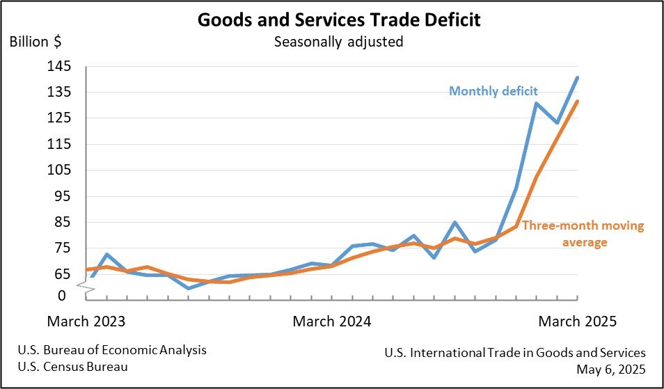
Table IIA-2B provides the US international trade balance, exports and imports of goods and services on an annual basis from 1960 to 2019. The trade balance deteriorated sharply over the long term. The US has a large deficit in goods or exports less imports of goods but it has a surplus in services that helps to reduce the trade account deficit or exports less imports of goods and services. The current account deficit at 2.8 percent in IVQ2018 decreases to 2.6 percent in IQ2019. The current account deficit decreases to 2.4 percent in IIQ2019. The current account deficit decreases to 2.3 percent in IIIQ2019. The current account deficit decreased to 2.0 percent in IVQ2019. The absolute value of the net international investment position at $9.6 trillion in IVQ2018 increases to $10.2 trillion in IQ2018. The absolute value of the net international investment position increases at $10.6 trillion in IIQ2019. The absolute value of the net international investment position increases to $10.98 trillion in IIIQ2019. The absolute value of the net international investment position increased to $10.99 trillion in IVQ2019. The ratio of the current account deficit to GDP has stabilized below 3 percent of GDP compared with much higher percentages before the recession but is combined now with much higher imbalance in the Treasury budget (see Pelaez and Pelaez, The Global Recession Risk (2007), Globalization and the State, Vol. II (2008b), 183-94, Government Intervention in Globalization (2008c), 167-71). There is still a major challenge in the combined deficits in current account and in federal budgets. The final rows of Table IIA-2B show marginal improvement of the trade deficit from $554,522 million in 2011 to lower $525,906 million in 2012 with exports growing 4.8 percent and imports 2.8 percent. The trade balance improved further to deficit of $446,829 million in 2013 with growth of exports of 2.9 percent while imports virtually stagnated, decreasing 0.5 percent. The trade deficit deteriorated in 2014 to $484,144 million with growth of exports of 3.4 percent and of imports of 4.2 percent. The trade deficit deteriorated in 2015 to $491,261 million with decrease of exports of 4.7 percent and decrease of imports of 3.7 percent. The trade deficit improved in 2016 to $481,169 million with decrease of exports of 1.8 percent and decrease of imports of 1.9 percent. The trade deficit deteriorated in 2017 to $513,791 million with growth of exports of 6.7 percent and of imports of 6.7 percent. The trade deficit deteriorated in 2018 to $579,937 million with growth of exports of 6.4 percent and of imports of 7.5 percent. The trade deficit improved in 2019 to $576,865 million with decrease of exports of 0.4 percent and decrease of imports of 0.5 percent. Growth and commodity shocks under alternating inflation waves (https://cmpassocregulationblog.blogspot.com/2020/09/wealth-of-households-and-nonprofit.html and earlier https://cmpassocregulationblog.blogspot.com/2020/08/d-ollar-devaluation-and-yuan.html) have deteriorated the trade deficit from the low of $394,771 million in 2009.

Table IIA-2B, US, International Trade Balance of Goods and Services, Exports and Imports of Goods and Services, SA, Millions of Dollars, Balance of Payments Basis

	Balance	Exports	∆%	Imports	∆%
1960	3,508	25,939		22,433
1961	4,194	26,403	1.8	22,208	-1.0
1962	3,371	27,722	5.0	24,352	9.7
1963	4,210	29,620	6.8	25,411	4.3
1964	6,022	33,340	12.6	27,319	7.5
1965	4,664	35,285	5.8	30,621	12.1
1966	2,939	38,926	10.3	35,987	17.5
1967	2,604	41,333	6.2	38,729	7.6
1968	250	45,544	10.2	45,292	16.9
1969	90	49,220	8.1	49,130	8.5
1970	2,255	56,640	15.1	54,385	10.7
1971	-1,301	59,677	5.4	60,980	12.1
1972	-5,443	67,223	12.6	72,664	19.2
1973	1,900	91,242	35.7	89,342	23.0
1974	-4,293	120,897	32.5	125,189	40.1
1975	12,403	132,585	9.7	120,181	-4.0
1976	-6,082	142,716	7.6	148,798	23.8
1977	-27,247	152,302	6.7	179,547	20.7
1978	-29,763	178,428	17.2	208,191	16.0
1979	-24,566	224,132	25.6	248,696	19.5
1980	-19,407	271,835	21.3	291,242	17.1
1981	-16,172	294,399	8.3	310,570	6.6
1982	-24,156	275,235	-6.5	299,392	-3.6
1983	-57,767	266,106	-3.3	323,874	8.2
1984	-109,074	291,094	9.4	400,166	23.6
1985	-121,879	289,071	-0.7	410,951	2.7
1986	-138,539	310,034	7.3	448,572	9.2
1987	-151,683	348,869	12.5	500,553	11.6
1988	-114,566	431,150	23.6	545,714	9.0
1989	-93,142	487,003	13.0	580,145	6.3
1990	-80,865	535,234	9.9	616,098	6.2
1991	-31,136	578,343	8.1	609,479	-1.1
1992	-39,212	616,882	6.7	656,094	7.6
1993	-70,311	642,863	4.2	713,174	8.7
1994	-98,493	703,254	9.4	801,747	12.4
1995	-96,384	794,387	13.0	890,771	11.1
1996	-104,065	851,602	7.2	955,667	7.3
1997	-108,273	934,453	9.7	1,042,726	9.1
1998	-166,140	933,174	-0.1	1,099,314	5.4
1999	-255,809	976,525	4.6	1,232,335	12.1
2000	-369,686	1,082,963	10.9	1,452,650	17.9
2001	-360,373	1,015,366	-6.2	1,375,739	-5.3
2002	-420,666	986,095	-2.9	1,406,762	2.3
2003	-496,243	1,028,186	4.3	1,524,429	8.4
2004	-610,838	1,168,120	13.6	1,778,958	16.7
2005	-716,542	1,291,503	10.6	2,008,045	12.9
2006	-763,533	1,463,991	13.4	2,227,523	10.9
2007	-710,997	1,660,815	13.4	2,371,811	6.5
2008	-712,350	1,849,586	11.4	2,561,936	8.0
2009	-394,771	1,592,792	-13.9	1,987,563	-22.4
2010	-503,087	1,872,320	17.5	2,375,407	19.5
2011	-554,522	2,143,552	14.5	2,698,074	13.6
2012	-525,906	2,247,453	4.8	2,773,359	2.8
2013	-446,829	2,313,237	2.9	2,760,066	-0.5
2014	-484,144	2,392,268	3.4	2,876,412	4.2
2015	-491,261	2,279,743	-4.7	2,771,004	-3.7
2016	-481,169	2,237,923	-1.8	2,719,092	-1.9
2017	-513,791	2,387,391	6.7	2,901,181	6.7
2018	-579,937	2,539,383	6.4	3,119,320	7.5
2019	-576,865	2,528,262	-0.4	3,105,127	-0.5

Source: US Census Bureau

Chart IIA-2 of the US Census Bureau provides the US trade account in goods and services SA from Jan 1992 to Aug 2020. There is long-term trend of deterioration of the US trade deficit shown vividly by Chart IIA-2. The global recession from IVQ2007 to IIQ2009 reversed the trend of deterioration. Deterioration resumed together with incomplete recovery and was influenced significantly by the carry trade from zero interest rates to commodity futures exposures (these arguments are elaborated in Pelaez and Pelaez, Financial Regulation after the Global Recession (2009a), 157-66, Regulation of Banks and Finance (2009b), 217-27, International Financial Architecture (2005), 15-18, The Global Recession Risk (2007), 221-5, Globalization and the State Vol. II (2008b), 197-213, Government Intervention in Globalization (2008c), 182-4 http://cmpassocregulationblog.blogspot.com/2011/07/causes-of-2007-creditdollar-crisis.html http://cmpassocregulationblog.blogspot.com/2011/01/professor-mckinnons-bubble-economy.html http://cmpassocregulationblog.blogspot.com/2011/01/world-inflation-quantitative-easing.html http://cmpassocregulationblog.blogspot.com/2011/01/treasury-yields-valuation-of-risk.html http://cmpassocregulationblog.blogspot.com/2010/11/quantitative-easing-theory-evidence-and.html http://cmpassocregulationblog.blogspot.com/2010/12/is-fed-printing-money-what-are.html). Earlier research focused on the long-term external imbalance of the US in the form of trade and current account deficits (Pelaez and Pelaez, The Global Recession Risk (2007), Globalization and the State Vol. II (2008b) 183-94, Government Intervention in Globalization (2008c), 167-71). US external imbalances have not been fully resolved and tend to widen together with improving world economic activity and commodity price shocks. There are additional effects for devaluation of the dollar with the Fed orienting interest increases now followed by decreases and inaction at near zero interest rates while the European Central Bank and the Bank of Japan determine negative nominal interest rates.

Chart IIA-2, US, Balance of Trade SA, Monthly, Millions of Dollars, Jan 1992-Aug 2020

Source: US Census Bureau

Char IIA-2A provides the US trade balance showing sharp deterioration in the global recession, with output in the US reaching a high in Feb 2020 (https://www.nber.org/cycles.html), in the lockdown of economic activity in the COVID-19 event.

Chart IIA-2A, US, Balance of Trade SA, Monthly, Millions of Dollars, Jan 2019-Aug 2020

Source: US Census Bureau

Chart IIA-3 of the US Census Bureau provides US exports SA from Jan 1992 to Aug 2020. There was sharp acceleration from 2003 to 2007 during worldwide economic boom and increasing inflation. Exports fell sharply during the financial crisis and global recession from IVQ2007 to IIQ2009. Growth picked up again together with world trade and inflation but stalled in the final segment with less rapid global growth and inflation. Exports contracted sharply in Mar-May 2020 in the global recession, with output in the US reaching a high in Feb 2020 (https://www.nber.org/cycles.html), in the lockdown of economic activity in the COVID-19 event with partial recovery in Jun-Aug 2020.

Chart IIA-3, US, Exports SA, Monthly, Millions of Dollars Jan 1992-Aug 2020

Source: US Census Bureau

Chart IIA-3A shows she sharp contraction of US exports in Mar-May 2020 followed by milder recovery in Jun-Aug 2020.

Chart IIA-3A, US, Exports SA, Monthly, Millions of Dollars Jan 2019-Aug 2020

Source: US Census Bureau

Growth was stronger between 2003 and 2007 with worldwide economic boom and inflation. There was sharp drop during the financial crisis and global recession. There is stalling import levels in the final segment in Chart IIA-4 resulting from weaker world economic growth and diminishing inflation because of risk aversion and portfolio reallocations from commodity exposures to equities. Imports contracted sharply in the global recession, with output in the US reaching a high in Feb 2020 (https://www.nber.org/cycles.html), in the lockdown of economic activity in the COVID-19 event with partial recovery in Jun-Aug 2020.

Chart IIA-4, US, Imports SA, Monthly, Millions of Dollars Jan 1992-Aug 2020

Source: US Census Bureau

Chart IIA-4A shows the sharp contraction of imports in Jan-May 2020 with recovery in Jun-Aug 2020.

Chart IIA-4A, US, Imports SA, Monthly, Millions of Dollars Jan 2019-Aug 2020

Source: US Census Bureau

There is deterioration of the US trade balance in goods in Table IIA-3 from deficit of $74,598 million in Aug 2019 to deficit of $83,860 million in Aug 2020. The nonpetroleum deficit increased from $72,649 million in Aug 2019 to $84,644 million in Aug 2020 while the petroleum deficit decreased from minus $1,014 million in Aug 2019 to $1,531 million in Aug 2020. Total exports of goods decreased 13.3 percent in Aug 2020 relative to a year earlier while total imports decreased 4.2 percent. Nonpetroleum exports decreased 11.4 percent from Aug 2019 to Aug 2020 while nonpetroleum imports decreased 1.0 percent. Petroleum imports decreased 41.0 percent with declining oil prices. Oil use contracted in the global recession, with output in the US reaching a high in Feb 2020 (https://www.nber.org/cycles.html), in the lockdown of economic activity in the COVID-19 event.

Table IIA-3, US, International Trade in Goods Balance, Exports and Imports $ Millions and ∆% SA

	Aug 2020	Aug 2019	∆%
Total Balance	-83,860	-74,598
Petroleum	1,531	-1,014
Non-Petroleum	-84,644	-72,649
Total Exports	119,099	137,358	-13.3
Petroleum	10,787	14,689	-26.6
Non-Petroleum	107,963	121,881	-11.4
Total Imports	202,959	211,956	-4.2
Petroleum	9,257	15,702	-41.0
Non-Petroleum	192,607	194,530	-1.0

Details may not add because of rounding and seasonal adjustment

Source: US Census Bureau

US exports and imports of goods not seasonally adjusted in Jan-Aug 2020 and Jan-Aug 2019 are in Table IIA-4. The rate of growth of exports was minus 16.1 percent and minus 11.2 percent for imports. The US has partial hedge of commodity price increases in exports of agricultural commodities that decreased 3.2 percent and of mineral fuels that decreased 20.5 percent both because prices of raw materials and commodities increase and fall recurrently because of shocks of risk aversion and portfolio reallocations. There is now the impact in the global recession, with output in the US reaching a high in Feb 2020 (https://www.nber.org/cycles.html), in the lockdown of economic activity in the COVID-19 event. The US exports a growing amount of crude oil, decreasing 23.2 percent in cumulative Jan-Aug 2020 relative to a year earlier. US exports and imports consist mostly of manufactured products, with less rapidly increasing prices. US manufactured exports decreased 17.3 percent while manufactured imports decreased 9.4 percent. Significant part of the US trade imbalance originates in imports of mineral fuels decreasing 41.4 percent and petroleum decreasing 42.0 percent with wide oscillations in oil prices. The limited hedge in exports of agricultural commodities and mineral fuels compared with substantial imports of mineral fuels and crude oil results in waves of deterioration of the terms of trade of the US, or export prices relative to import prices, originating in commodity price increases caused by carry trades from zero interest rates. These waves are similar to those in worldwide inflation.

Table IIA-4, US, Exports and Imports of Goods, Not Seasonally Adjusted Millions of Dollars and %, Census Basis

	Jan-Aug 2020 $ Millions	Jan-Aug 2019 $ Millions	∆%
Exports	918,034	1,094,383	-16.1
Manufactured	622,717	753,066	-17.3
Agricultural Commodities	87,026	89,862	-3.2
Mineral Fuels	102,205	128,510	-20.5
Petroleum	77,957	101,459	-23.2
Imports	1,482,512	1,669,627	-11.2
Manufactured	1,306,618	1,442,571	-9.4
Agricultural Commodities	90,333	89,085	1.4
Mineral Fuels	81,517	139,155	-41.4
Petroleum	75,956	131,064	-42.0

Source: US Census Bureau

Table IIA-4A provides the United States balance of trade in goods, exports of goods and imports of goods NSA in millions of US dollars and percent share in Jan-Aug 2020. North America, consisting of Mexico and Canada, have joint share of 32.4 percent of exports and 25.3 percent of imports. The combined share of North America and Europe is 56.1 percent of exports and 50.8 percent of imports. The share of the Pacific Rim in exports is 25.8 percent and 34.6 percent of imports.

Table IIA-4A United States, Balance of Trade in Goods, Exports in Goods and Imports of Goods, NSA, Millions of US Dollars

Jan-Aug 2020	Millions USD	Million USD	Percent	Million USD	Percent
Region/Country	Balance	Exports		Imports
Total Census Basis	-564,478	918,034		1,482,512
North America*	-77,464	297,643	32.4	375,107	25.3
Europe	-160,122	217,629	23.7	377,751	25.5
Euro Area	-96,082	139,832	15.2	235,914	15.9
Pacific Rim	-276,843	236,759	25.8	513,603	34.6
China	-193,117	69,564	7.6	262,681	17.7
Japan	-31,901	43,243	4.7	75,144	5.1
Brazil	7,932	22,577	2.5	14,645	1.0

*Canada and Mexico

Source: US Census Bureau

https://apps.bea.gov/iTable/iTable.cfm?reqid=19&step=3&isuri=1&1921=survey&1903=46#reqid=19&step=3&isuri=1&1921=survey&1903=46

IID. United States International Terms of Trade. Delfim Netto (1959) partly reprinted in Pelaez (1973) conducted two classical nonparametric tests (Mann 1945, Wallis and Moore 1941; see Kendall and Stuart 1968) with coffee-price data in the period of free markets from 1857 to 1906 with the following conclusions (Pelaez, 1976a, 280):

“First, the null hypothesis of no trend was accepted with high confidence; secondly, the null hypothesis of no oscillation was rejected also with high confidence. Consequently, in the nineteenth century international prices of coffee fluctuated but without long-run trend. This statistical fact refutes the extreme argument of structural weakness of the coffee trade.”

In his classic work on the theory of international trade, Jacob Viner (1937, 563) analyzed the “index of total gains from trade,” or “amount of gain per unit of trade,” denoted as T:

T= (∆P^e/∆Pⁱ)∆Q

Where ∆P^e is the change in export prices, ∆Pⁱ is the change in import prices and ∆Q is the change in export volume. Dorrance (1948, 52) restates “Viner’s index of total gain from trade” as:

“What should be done is to calculate an index of the value (quantity multiplied by price) of exports and the price of imports for any country whose foreign accounts are to be analysed. Then the export value index should be divided by the import price index. The result would be an index which would reflect, for the country concerned, changes in the volume of imports obtainable from its export income (i.e. changes in its "real" export income, measured in import terms). The present writer would suggest that this index be referred to as the ‘income terms of trade’ index to differentiate it from the other indexes at present used by economists.”

What really matters for an export activity especially during modernization is the purchasing value of goods that it exports in terms of prices of imports. For a primary producing country, the purchasing power of exports in acquiring new technology from the country providing imports is the critical measurement. The barter terms of trade of Brazil improved from 1857 to 1906 because international coffee prices oscillated without trend (Delfim Netto 1959) while import prices from the United Kingdom declined at the rate of 0.5 percent per year (Imlah 1958). The accurate measurement of the opportunity afforded by the coffee exporting economy was incomparably greater when considering the purchasing power in British prices of the value of coffee exports, or Dorrance’s (1948) income terms of trade.

The conventional theory that the terms of trade of Brazil deteriorated over the long term is without reality (Pelaez 1976a, 280-281):

“Moreover, physical exports of coffee by Brazil increased at the high average rate of 3.5 per cent per year. Brazil's exchange receipts from coffee-exporting in sterling increased at the average rate of 3.5 per cent per year and receipts in domestic currency at 4.5 per cent per year. Great Britain supplied nearly all the imports of the coffee economy. In the period of the free coffee market, British export prices declined at the rate of 0.5 per cent per year. Thus, the income terms of trade of the coffee economy improved at the relatively satisfactory average rate of 4.0 per cent per year. This is only a lower bound of the rate of improvement of the terms of trade. While the quality of coffee remained relatively constant, the quality of manufactured products improved significantly during the fifty-year period considered. The trade data and the non-parametric tests refute conclusively the long-run hypothesis. The valid historical fact is that the tropical export economy of Brazil experienced an opportunity of absorbing rapidly increasing quantities of manufactures from the "workshop" countries. Therefore, the coffee trade constituted a golden opportunity for modernization in nineteenth-century Brazil.”

Imlah (1958) provides decline of British export prices at 0.5 percent in the nineteenth century and there were no lost decades, depressions or unconventional monetary policies in the highly dynamic economy of England that drove the world’s growth impulse. Inflation in the United Kingdom between 1857 and 1906 is measured by the composite price index of O’Donoghue and Goulding (2004) at minus 7.0 percent or average rate of decline of 0.2 percent per year.

Simon Kuznets (1971) analyzes modern economic growth in his Lecture in Memory of Alfred Nobel:

“The major breakthroughs in the advance of human knowledge, those that constituted dominant sources of sustained growth over long periods and spread to a substantial part of the world, may be termed epochal innovations. And the changing course of economic history can perhaps be subdivided into economic epochs, each identified by the epochal innovation with the distinctive characteristics of growth that it generated.Without considering the feasibility of identifying and dating such economic epochs, we may proceed on the working assumption that modern economic growth represents such a distinct epoch - growth dating back to the late eighteenth century and limited (except in significant partial effects) to economically developed countries. These countries, so classified because they have managed to take adequate advantage of the potential of modern technology, include most of Europe, the overseas offshoots of Western Europe, and Japan—barely one quarter of world population.”

Cameron (1961) analyzes the mechanism by which the Industrial Revolution in Great Britain spread throughout Europe and Cameron (1967) analyzes the financing by banks of the Industrial Revolution in Great Britain. O’Donoghue and Goulding (2004) provide consumer price inflation in England since 1750 and MacFarlane and Mortimer-Lee (1994) analyze inflation in England over 300 years. Lucas (2004) estimates world population and production since the year 1000 with sustained growth of per capita incomes beginning to accelerate for the first time in English-speaking countries and in particular in the Industrial Revolution in Great Britain. The conventional theory is unequal distribution of the gains from trade and technical progress between the industrialized countries and developing economies (Singer 1950, 478):

“Dismissing, then, changes in productivity as a governing factor in changing terms of trade, the following explanation presents itself: the fruits of technical progress may be distributed either to producers (in the form of rising incomes) or to consumers (in the form of lower prices). In the case of manufactured commodities produced in more developed countries, the former method, i.e., distribution to producers through higher incomes, was much more important relatively to the second method, while the second method prevailed more in the case of food and raw material production in the underdeveloped countries. Generalizing, we may say -that technical progress in manufacturing industries showed in a rise in incomes while technical progress in the production of food and raw materials in underdeveloped countries showed in a fall in prices”

Temin (1997, 79) uses a Ricardian trade model to discriminate between two views on the Industrial Revolution with an older view arguing broad-based increases in productivity and a new view concentration of productivity gains in cotton manufactures and iron:

“Productivity advances in British manufacturing should have lowered their prices relative to imports. They did. Albert Imlah [1958] correctly recognized this ‘severe deterioration’ in the net barter terms of trade as a signal of British success, not distress. It is no surprise that the price of cotton manufactures fell rapidly in response to productivity growth. But even the price of woolen manufactures, which were declining as a share of British exports, fell almost as rapidly as the price of exports as a whole. It follows, therefore, that the traditional ‘old-hat’ view of the Industrial Revolution is more accurate than the new, restricted image. Other British manufactures were not inefficient and stagnant, or at least, they were not all so backward. The spirit that motivated cotton manufactures extended also to activities as varied as hardware and haberdashery, arms, and apparel.”

Phyllis Deane (1968, 96) estimates growth of United Kingdom gross national product (GNP) at around 2 percent per year for several decades in the nineteenth century. The facts that the terms of trade of Great Britain deteriorated during the period of epochal innovation and high rates of economic growth while the income terms of trade of the coffee economy of nineteenth-century Brazil improved at the average yearly rate of 4.0 percent from 1857 to 1906 disprove the hypothesis of weakness of trade as an explanation of relatively lower income and wealth. As Temin (1997) concludes, Britain did pass on lower prices and higher quality the benefits of technical innovation. Explanation of late modernization must focus on laborious historical research on institutions and economic regimes together with economic theory, data gathering and measurement instead of grand generalizations of weakness of trade and alleged neocolonial dependence (Stein and Stein 1970, 134-5):

“Great Britain, technologically and industrially advanced, became as important to the Latin American economy as to the cotton-exporting southern United States. [After Independence in the nineteenth century] Latin America fell back upon traditional export activities, utilizing the cheapest available factor of production, the land, and the dependent labor force.”

Summerhill (2015) contributes momentous solid facts and analysis with an ideal method combining economic theory, econometrics, international comparisons, data reconstruction and exhaustive archival research. Summerhill (2015) finds that Brazil committed to service of sovereign foreign and internal debt. Contrary to conventional wisdom, Brazil generated primary fiscal surpluses during most of the Empire until 1889 (Summerhill 2015, 37-8, Figure 2.1). Econometric tests by Summerhill (2015, 19-44) show that Brazil’s sovereign debt was sustainable. Sovereign credibility in the North-Weingast (1989) sense spread to financial development that provided the capital for modernization in England and parts of Europe (see Cameron 1961, 1967). Summerhill (2015, 3, 194-6, Figure 7.1) finds that “Brazil’s annual cost of capital in London fell from a peak of 13.9 percent in 1829 to only 5.12 percent in 1889. Average rates on secured loans in the private sector in Rio, however, remained well above 12 percent through 1850.” Financial development would have financed diversification of economic activities, increasing productivity and wages and ensuring economic growth. Brazil restricted creation of limited liability enterprises (Summerhill 2015, 151-82) that prevented raising capital with issue of stocks and corporate bonds. Cameron (1961) analyzed how the industrial revolution in England spread to France and then to the rest of Europe. The Société Générale de Crédit Mobilier of Émile and Isaac Péreire provided the “mobilization of credit” for the new economic activities (Cameron 1961). Summerhill (2015, 151-9) provides facts and analysis demonstrating that regulation prevented the creation of a similar vehicle for financing modernization by Irineu Evangelista de Souza, the legendary Visconde de Mauá. Regulation also prevented the use of negotiable bearing notes of the Caisse Générale of Jacques Lafitte (Cameron 1961, 118-9). The government also restricted establishment and independent operation of banks (Summerhill 2015, 183-214). Summerhill (2015, 198-9) measures concentration in banking that provided economic rents or a social loss. The facts and analysis of Summerhill (2015) provide convincing evidence in support of the economic theory of regulation, which postulates that regulated entities capture the process of regulation to promote their self-interest. There appears to be a case that excessively centralized government can result in regulation favoring private instead of public interests with adverse effects on economic activity. The contribution of Summerhill (2015) explains why Brazil did not benefit from trade as an engine of growth—as did regions of recent settlement in the vision of nineteenth-century trade and development of Ragnar Nurkse (1959)—partly because of restrictions on financing and incorporation. Professor Rondo E. Cameron, in his memorable A Concise Economic History of the World (Cameron 1989, 307-8), finds that “from a broad spectrum of possible forms of interaction between the financial sector and other sectors of the economy that requires its services, one can isolate three type-cases: (1) that in which the financial sector plays a positive, growth-inducing role; (2) that in which the financial sector is essentially neutral or merely permissive; and (3) that in which inadequate finance restricts or hinders industrial and commercial development.” Summerhill (2015) proves exhaustively that Brazil failed to modernize earlier because of the restrictions of an inadequate institutional financial arrangement plagued by regulatory capture for self-interest.

There is analysis of the origins of current tensions in the world economy (Pelaez and Pelaez, Financial Regulation after the Global Recession (2009a), Regulation of Banks and Finance (2009b), International Financial Architecture (2005), The Global Recession Risk (2007), Globalization and the State Vol. I (2008a), Globalization and the State Vol. II (2008b), Government Intervention in Globalization (2008c)).

The US Bureau of Economic Analysis (BEA) measures the terms of trade index of the United States quarterly since 1947 and annually since 1929. Chart IID-1 provides the terms of trade of the US quarterly since 1947 with significant long-term deterioration from 150.474 in IQ1947 to 107.721 in IIQ2020, decreasing from 109.980 in IVQ2019 and increasing from 109.680 in IQ2020. Significant part of the deterioration occurred from the 1960s to the 1980s followed by some recovery and then stability.

Chart IID-1, United States Terms of Trade Quarterly Index 1947-2020

Source: Bureau of Economic Analysis

Chart IID-1A provides the annual US terms of trade from 1929 to 2019. The index fell from 142.590 in 1929 to 109.740 in 2019. There is decline from 1971 to a much lower plateau.

Chart IID-1A, United States Terms of Trade Annual Index 1929-2019, Annual

Source: Bureau of Economic Analysis

https://apps.bea.gov/iTable/iTable.cfm?reqid=19&step=3&isuri=1&1921=survey&1903=46#reqid=19&step=3&isuri=1&1921=survey&1903=46

Chart IID-1B provides the US terms of trade index, index of terms of trade of nonpetroleum goods and index of terms of trade of goods. The terms of trade of nonpetroleum goods dropped sharply from the mid-1980s to 1995, recovering significantly until 2014, dropping and then recovering again into 2019. There is relative stability in the terms of trade of nonpetroleum goods from 1967 to 2019 but sharp deterioration in the overall index and the index of goods.

Chart IID-1B, United States Terms of Trade Annual Indexes 1967-2019, Annual

Source: Bureau of Economic Analysis

https://apps.bea.gov/iTable/iTable.cfm?reqid=19&step=3&isuri=1&1921=survey&1903=46#reqid=19&step=3&isuri=1&1921=survey&1903=46

The US Bureau of Labor Statistics (BLS) provides measurements of US international terms of trade. The measurement by the BLS is as follows (https://www.bls.gov/mxp/terms-of-trade.htm):

“BLS terms of trade indexes measure the change in the U.S. terms of trade with a specific country, region, or grouping over time. BLS terms of trade indexes cover the goods sector only.

To calculate the U.S. terms of trade index, take the U.S. all-export price index for a country, region, or grouping, divide by the corresponding all-import price index and then multiply the quotient by 100. Both locality indexes are based in U.S. dollars and are rounded to the tenth decimal place for calculation. The locality indexes are normalized to 100.0 at the same starting point.
TT_t=(LOD_t/LOO_t)*100,
where
TT_t=Terms of Trade Index at time t
LOD_t=Locality of Destination Price Index at time t
LOO_t=Locality of Origin Price Index at time t
The terms of trade index measures whether the U.S. terms of trade are improving or deteriorating over time compared to the country whose price indexes are the basis of the comparison. When the index rises, the terms of trade are said to improve; when the index falls, the terms of trade are said to deteriorate. The level of the index at any point in time provides a long-term comparison; when the index is above 100, the terms of trade have improved compared to the base period, and when the index is below 100, the terms of trade have deteriorated compared to the base period.”

Chart IID-3 provides the BLS terms of trade of the US with Canada. The index increases from 100.0 in Dec 2017 to 117.8 in Dec 2018 and decreases to 104.0 in Feb 2020. The index increases to 121.5 in Apr 2020. The index decreased to 101.6 in Aug 2020.

Chart IID-3, US Terms of Trade, Monthly, All Goods, Canada, NSA, Dec 2017=100

Source: Bureau of Labor Statistics https://www.bls.gov/mxp/data.htm

Chart IID-4 provides the BLS terms of trade of the US with the European Union. There is improvement from 100.0 in Dec 2017 to 102.8 in Jan 2020 followed by decrease to 100.2 in Aug 2020.

Chart IID-4, US Terms of Trade, Monthly, All Goods, European Union, NSA, Dec 2017=100

Source: Bureau of Labor Statistics https://www.bls.gov/mxp/data.htm

Chart IID-4 provides the BLS terms of trade of the US with Mexico. There is deterioration from 100.0 in Dec 2017 to 96.8 in Aug 2020.

Chart IID-5, US Terms of Trade, Monthly, All Goods, Mexico, NSA, Dec 2017=100

Source: Bureau of Labor Statistics https://www.bls.gov/mxp/data.htm

Chart IID-4 provides the BLS terms of trade of the US with China. There is deterioration from 100.0 in Dec 2017 to 98.0 in Sep 2018, improvement to 100.6 in Apr 2019 with deterioration to 99.4 in Aug 2020.

Chart IID-6, US Terms of Trade, Monthly, All Goods, China, NSA, Dec 2017=100

Source: Bureau of Labor Statistics https://www.bls.gov/mxp/data.htm

Chart IID-4 provides the BLS terms of trade of the US with Japan. There is deterioration from 100.0 in Dec 2017 to 99.2 in Dec 2019 and deterioration to 97.0 in Aug 2020.

Chart IID-7, US Terms of Trade, Monthly, All Goods, Japan, NSA, Dec 2017=100

Source: Bureau of Labor Statistics https://www.bls.gov/mxp/data.htm

Manufacturing is underperforming in the lost cycle of the global recession. Manufacturing (NAICS) in Aug 2020 is lower by 9.1 percent relative to the peak in Jun 2007, as shown in Chart V-3A. Manufacturing (SIC) in Aug 2020 at 99.2841 is lower by 11.6 percent relative to the peak at 112.3113 in Jun 2007. There is cyclical uncommonly slow growth in the US instead of allegations of secular stagnation. There is similar behavior in manufacturing. There is classic research on analyzing deviations of output from trend (see for example Schumpeter 1939, Hicks 1950, Lucas 1975, Sargent and Sims 1977). The long-term trend is growth of manufacturing at average 2.9 percent per year from Aug 1919 to Aug 2020. Growth at 2.9 percent per year would raise the NSA index of manufacturing output (SIC, Standard Industrial Classification) from 108.2987 in Dec 2007 to 155.5554 in Aug 2020. The actual index NSA in Aug 2020 is 99.2841 which is 36.2 percent below trend. The underperformance of manufacturing in Mar-Aug 2020 originates partly in the earlier global recession augmented by the current global recession with output in the US reaching a high in Feb 2020 (https://www.nber.org/cycles.html), in the lockdown of economic activity in the COVID-19. Manufacturing grew at the average annual rate of 3.3 percent between Dec 1986 and Dec 2006. Growth at 3.3 percent per year would raise the NSA index of manufacturing output (SIC, Standard Industrial Classification) from 108.2987 in Dec 2007 to 163.3909 in Aug 2020. The actual index NSA in Aug 2020 is 99.2841, which is 39.2 percent below trend. Manufacturing output grew at average 1.7 percent between Dec 1986 and Aug 2020. Using trend growth of 1.7 percent per year, the index would increase to 134.0774 in Aug 2020. The output of manufacturing at 99.2841 in Aug 2020 is 26.0 percent below trend under this alternative calculation. Using the NAICS (North American Industry Classification System), manufacturing output fell from the high of 110.5147 in Jun 2007 to the low of 86.3800 in Apr 2009 or 21.8 percent. The NAICS manufacturing index increased from 86.3800 in Apr 2009 to 100.4257 in Aug 2020 or 16.3 percent. The NAICS manufacturing index increased at the annual equivalent rate of 3.5 percent from Dec 1986 to Dec 2006. Growth at 3.5 percent would increase the NAICS manufacturing output index from 106.6777 in Dec 2007 to 164.9372 in Aug 2020. The NAICS index at 100.4257 in Aug 2020 is 39.1 below trend. The NAICS manufacturing output index grew at 1.7 percent annual equivalent from Dec 1999 to Dec 2006. Growth at 1.7 percent would raise the NAICS manufacturing output index from 106.6777 in Dec 2007 to 132.0705 in Aug 2020. The NAICS index at 100.4257 in Aug 2020 is 24.0 percent below trend under this alternative calculation.

Chart V-3A, United States Manufacturing NSA, Dec 2007 to Aug 2020

Board of Governors of the Federal Reserve System

https://www.federalreserve.gov/releases/g17/Current/default.htm

Chart V-3A, United States Manufacturing (NAICS) NSA, Jun 2007 to Aug 2020

Board of Governors of the Federal Reserve System

https://www.federalreserve.gov/releases/g17/Current/default.htm

Chart V-3B provides the civilian noninstitutional population of the United States, or those available for work. The civilian noninstitutional population increased from 231.713 million in Jun 2007 to 260.558 million in Aug 2020 or 28.845 million.

Chart V-3B, United States, Civilian Noninstitutional Population, Million, NSA, Jan 2007 to Aug 2020

Source: US Bureau of Labor Statistics

Chart V-3C provides nonfarm payroll manufacturing jobs in the United States from Jan 2007 to Jul 2020. Nonfarm payroll manufacturing jobs fell from 13.987 million in Aug 2007 to 12.211 million in Aug 2020, or 1.776 million.

Chart V-3C, United States, Payroll Manufacturing Jobs, NSA, Jan 2007 to Aug 2020, Thousands

Source: US Bureau of Labor Statistics

https://www.federalreserve.gov/releases/g17/Current/default.htm

Chart V-3D provides the index of US manufacturing (NAICS) from Jan 1972 to Aug 2020. The index continued increasing during the decline of manufacturing jobs after the early 1980s. There are likely effects of changes in the composition of manufacturing with also changes in productivity and trade. There is sharp decline in the global recession, with output in the US reaching a high in Feb 2020 (https://www.nber.org/cycles.html), in the lockdown of economic activity in the COVID-19 event. There is initial recovery in May-Aug 2020.

Chart V-3D, United States Manufacturing (NAICS) NSA, Jan 1972 to Aug 2020

Source: Board of Governors of the Federal Reserve System

Chart V-3E provides the US noninstitutional civilian population, or those in condition of working, from Jan 1948, when first available, to Aug 2020. The noninstitutional civilian population increased from 170.042 million in Jun 1981 to 260.558 million in Aug 2020, or 90.516 million.

Chart V-3E, United States, Civilian Noninstitutional Population, Million, NSA, Jan 1948 to Aug 2020

Source: US Bureau of Labor Statistics

Chart V-3F provides manufacturing jobs in the United States from Jan 1939 to May 2020. Nonfarm payroll manufacturing jobs decreased from a peak of 18.890 million in Jun 1981 to 12.211 million in Aug 2020.

Chart V-3C, United States, Payroll Manufacturing Jobs, NSA, Jan 1939 to Aug 2020, Thousands

Source: US Bureau of Labor Statistics