
CANNOT UPLOAD CHARTS AND IMAGES: ERROR 403
Recovery without Hiring, Ten Million Fewer Full-Time Jobs, Youth and Middle-Age Unemployment, United States Inflation, United States International Trade, United States Balance of Payments Current Account and Net International Investment Position, Collapse of United States Dynamism of Income Growth and Employment Creation in the Lost Economic Cycle of the Global Recession with Economic Growth Underperforming Below Trend Worldwide, World Financial Turbulence, World Cyclical Slow Growth, Government Intervention in Globalization, and Global Recession Risk
© Carlos M. Pelaez, 2009, 2010, 2011, 2012, 2013, 2014, 2015, 2016, 2017, 2018
I Recovery without Hiring
IA1 Hiring Collapse
IA2 Labor Underutilization
ICA3 Ten Million Fewer Full-time Jobs
IA4 Theory and Reality of Cyclical Slow Growth Not Secular Stagnation: Youth and Middle-Age Unemployment
II United States Inflation
IIB United States International Trade
IIC United States Balance of Payments Current Account and Net International Investment Position
II IB Collapse of United States Dynamism of Income Growth and Employment Creation in the Lost Economic Cycle of the Global Recession with Economic Growth Underperforming Below Trend Worldwide
III World Financial Turbulence
IV Global Inflation
V World Economic Slowdown
VA United States
VB Japan
VC China
VD Euro Area
VE Germany
VF France
VG Italy
VH United Kingdom
VI Valuation of Risk Financial Assets
VII Economic Indicators
VIII Interest Rates
IX Conclusion
References
Appendixes
Appendix I The Great Inflation
IIIB Appendix on Safe Haven Currencies
IIIC Appendix on Fiscal Compact
IIID Appendix on European Central Bank Large Scale Lender of Last Resort
IIIG Appendix on Deficit Financing of Growth and the Debt Crisis
II United States Inflation. C Long-Term US Inflation. Key percentage average yearly rates of the US economy on growth and inflation are provided in Table I-1 updated with release of new data. The choice of dates prevents the measurement of long-term potential economic growth because of two recessions from IQ2001 (Mar) to IVQ2001 (Nov) with decline of GDP of 0.3 percent and the drop in GDP of 4.2 percent in the recession from IVQ2007 (Dec) to IIQ2009 (June) (https://cmpassocregulationblog.blogspot.com/2018/06/fluctuating-valuations-of-risk.html and earlier https://cmpassocregulationblog.blogspot.com/2018/06/stronger-dollar-mediocre-cyclical.html). Long-term economic performance in the United States consisted of trend growth of GDP at 3 percent per year and of per capita GDP at 2 percent per year as measured for 1870 to 2010 by Robert E Lucas (2011May). The economy returned to trend growth after adverse events such as wars and recessions. The key characteristic of adversities such as recessions was much higher rates of growth in expansion periods that permitted the economy to recover output, income and employment losses that occurred during the contractions. Over the business cycle, the economy compensated the losses of contractions with higher growth in expansions to maintain trend growth of GDP of 3 percent and of GDP per capita of 2 percent. The US maintained growth at 3.0 percent on average over entire cycles with expansions at higher rates compensating for contractions. Key percentage average yearly rates of the US economy on growth and inflation are provided in Table I-1 updated with release of new data. US economic growth has been at only 2.2 percent on average in the cyclical expansion in the 35 quarters from IIIQ2009 to IQ2018. Boskin (2010Sep) measures that the US economy grew at 6.2 percent in the first four quarters and 4.5 percent in the first 12 quarters after the trough in the second quarter of 1975; and at 7.7 percent in the first four quarters and 5.8 percent in the first 12 quarters after the trough in the first quarter of 1983 (Professor Michael J. Boskin, Summer of Discontent, Wall Street Journal, Sep 2, 2010 http://professional.wsj.com/article/SB10001424052748703882304575465462926649950.html). There are new calculations using the revision of US GDP and personal income data since 1929 by the Bureau of Economic Analysis (BEA) (http://bea.gov/iTable/index_nipa.cfm) and the third estimate of GDP for IQ2018 (https://www.bea.gov/newsreleases/national/gdp/2018/pdf/gdp1q18_3rd.pdf). The average of 7.7 percent in the first four quarters of major cyclical expansions is in contrast with the rate of growth in the first four quarters of the expansion from IIIQ2009 to IIQ2010 of only 2.7 percent obtained by dividing GDP of $14,745.9 billion in IIQ2010 by GDP of $14,355.6 billion in IIQ2009 {[($14,745.9/$14,355.6) -1]100 = 2.7%], or accumulating the quarter on quarter growth rates (https://cmpassocregulationblog.blogspot.com/2018/06/fluctuating-valuations-of-risk.html and earlier https://cmpassocregulationblog.blogspot.com/2018/06/stronger-dollar-mediocre-cyclical.html). The expansion from IQ1983 to IVQ1985 was at the average annual growth rate of 5.9 percent, 5.4 percent from IQ1983 to IIIQ1986, 5.2 percent from IQ1983 to IVQ1986, 5.0 percent from IQ1983 to IQ1987, 5.0 percent from IQ1983 to IIQ1987, 4.9 percent from IQ1983 to IIIQ1987, 5.0 percent from IQ1983 to IVQ1987, 4.9 percent from IQ1983 to IIQ1988, 4.8 percent from IQ1983 to IIIQ1988, 4.8 percent from IQ1983 to IVQ1988, 4.8 percent from IQ1983 to IQ1989, 4.7 percent from IQ1983 to IIQ1989, 4.7 percent from IQ1983 to IIIQ1989, 4.5 percent from IQ1983 to IVQ1989. 4.5 percent from IQ1983 to IQ1990, 4.4 percent from IQ1983 to IIQ1990, 4.3 percent from IQ1983 to IIIQ1990, 4.0 percent from IQ1983 to IVQ1990, 3.8 percent from IQ1983 to IQ1991, 3.8 percent from IQ1983 to IIQ1991, 3.8 percent from IQ1983 to IIIQ1991 and at 7.8 percent from IQ1983 to IVQ1983 (https://cmpassocregulationblog.blogspot.com/2018/06/fluctuating-valuations-of-risk.html and earlier https://cmpassocregulationblog.blogspot.com/2018/06/stronger-dollar-mediocre-cyclical.html). The National Bureau of Economic Research (NBER) dates a contraction of the US from IQ1990 (Jul) to IQ1991 (Mar) (http://www.nber.org/cycles.html). The expansion lasted until another contraction beginning in IQ2001 (Mar). US GDP contracted 1.3 percent from the pre-recession peak of $8983.9 billion of chained 2009 dollars in IIIQ1990 to the trough of $8865.6 billion in IQ1991 (http://www.bea.gov/iTable/index_nipa.cfm). The US maintained growth at 3.0 percent on average over entire cycles with expansions at higher rates compensating for contractions. Growth at trend in the entire cycle from IVQ2007 to IQ2018 would have accumulated to 35.4 percent. GDP in IQ2018 would be $20,298.9 billion (in constant dollars of 2009) if the US had grown at trend, which is higher by $2927.0 billion than actual $17,371.9 billion. There are about two trillion dollars of GDP less than at trend, explaining the 20.6 million unemployed or underemployed equivalent to actual unemployment/underemployment of 12.1 percent of the effective labor force (https://cmpassocregulationblog.blogspot.com/2018/07/twenty-one-million-unemployed-or.html and earlier https://cmpassocregulationblog.blogspot.com/2018/06/twenty-one-million-unemployed-or.html). US GDP in IQ2018 is 14.4 percent lower than at trend. US GDP grew from $14,991.8 billion in IVQ2007 in constant dollars to $17,371.9 billion in IQ2018 or 15.9 percent at the average annual equivalent rate of 1.4 percent. Professor John H. Cochrane (2014Jul2) estimates US GDP at more than 10 percent below trend. Cochrane (2016May02) measures GDP growth in the US at average 3.5 percent per year from 1950 to 2000 and only at 1.76 percent per year from 2000 to 2015 with only at 2.0 percent annual equivalent in the current expansion. Cochrane (2016May02) proposes drastic changes in regulation and legal obstacles to private economic activity. The US missed the opportunity to grow at higher rates during the expansion and it is difficult to catch up because growth rates in the final periods of expansions tend to decline. The US missed the opportunity for recovery of output and employment always afforded in the first four quarters of expansion from recessions. Zero interest rates and quantitative easing were not required or present in successful cyclical expansions and in secular economic growth at 3.0 percent per year and 2.0 percent per capita as measured by Lucas (2011May). There is cyclical uncommonly slow growth in the US instead of allegations of secular stagnation. There is similar behavior in manufacturing. There is classic research on analyzing deviations of output from trend (see for example Schumpeter 1939, Hicks 1950, Lucas 1975, Sargent and Sims 1977). The long-term trend is growth of manufacturing at average 3.2 percent per year from May 1919 to May 2018. Growth at 3.2 percent per year would raise the NSA index of manufacturing output from 108.3221 in Dec 2007 to 150.3883 in May 2018. The actual index NSA in May 2018 is 103.9274, which is 30.9 percent below trend. Manufacturing output grew at average 1.9 percent between Dec 1986 and May 2018. Using trend growth of 1.9 percent per year, the index would increase to 131.7847 in May 2018. The output of manufacturing at 103.9274 in May 2018 is 21.1 percent below trend under this alternative calculation. The US maintained growth at 3.0 percent on average over entire cycles with expansions at higher rates compensating for contractions. In the period from 1929 to 2017 the average growth rate of real GDP was 3.2 percent and 3.2 percent between 1947 to 2017, which is close to 3.0 percent from 1870 to 2010 measured by Lucas (2011May), as shown in Table I-1. From 1929 to 2017, nominal GDP grew at the average rate of 6.1 percent and at 6.4 percent from 1947 to 2017. The implicit deflator increased at the average rate of 2.8 percent from 1929 to 2017 and at 3.2 percent from 1947 to 2017. Between 2000 and 2017, real GDP grew at the average rate of 1.8 percent per year, nominal GDP at 3.8 percent and the implicit deflator at 1.9 percent. The annual average rate of CPI increase was 3.1 percent from 1913 to 2017, 3.5 percent from 1947 to 2017 and 2.1 percent from 2000 to 2017. Between 2000 and 2017, the average rate of CPI inflation was 2.1 percent per year and 2.0 percent excluding food and energy. From 2000 to 2018, the average rate of CPI inflation was 2.1 percent and 2.0 percent excluding food and energy. The average annual rate of PPI inflation was 2.9 percent from 1947 to 2017 and 2.1 percent from 2000 to 2017. PPI inflation increased at 2.1 percent per year on average from 2000 to 2017, 2.2 percent on average from 2000 to 2018 and at 1.8 percent excluding food and energy from 2000 to 2017 and 1.8 percent from 2000 to 2018. Producer price inflation of finished energy goods increased at average 2.9 percent between 2000 and 2017 and at 3.5 percent between 2000 and 2018. There is also inflation in international trade. Import prices increased at 1.2 percent per year between 2000 and 2017 and 1.4 percent between 2000 and 2018. The commodity price shock is revealed by inflation of import prices of petroleum increasing at 3.4 percent per year between 2000 and 2017 and at 5.0 percent between 2000 and 2018. Import prices excluding petroleum increased at the average rate of 0.7 percent from 2000 to 2017 and at 0.7 percent from 2000 to 2018. The average percentage rates of increase of import prices excluding fuels are at 1.0 percent for 2002 to 2017 and 1.0 percent for 2002 to 2018. Export prices rose at the average rate of 1.2 percent between 2000 and 2017 and at 1.4 percent from 2000 to 2018. What spared the US of sharper decade-long deterioration of the terms of trade, (export prices)/(import prices), was its diversification and competitiveness in agriculture. Agricultural export prices grew at the average yearly rate of 3.3 percent from 2000 to 2017 and at 3.4 percent from 2000 to 2018. US nonagricultural export prices rose at 1.0 percent per year from 2000 to 2017 and at 1.2 percent from 2000 to 2018. The share of petroleum imports in US trade far exceeds that of agricultural exports. Unconventional monetary policy inducing carry trades in commodities has deteriorated US terms of trade, prices of exports relative to prices of imports, tending to restrict growth of US aggregate real income. These dynamic inflation rates are not similar to those for the economy of Japan where inflation was negative in seven of the 10 years in the 2000s. There is no reality of the proposition of need of unconventional monetary policy in the US because of deflation panic. There is reality in cyclical slow economic growth currently but not in secular stagnation.
Table I-1, US, Average Growth Rates of Real and Nominal GDP, Consumer Price Index, Producer Price Index and Import and Export Prices, Percent per Year
| Real GDP | 2000-2017: 1.8% 1929-2017: 3.2% 1947-2017: 3.2% |
| Nominal GDP | 2000-2017: 3.8% 1929-2017: 6.1% 1947-2017: 6.4% |
| Implicit Price Deflator | 2000-2017: 1.9% 1929-2017: 2.8% 1947-2017: 3.2% |
| CPI | 2000-2017: 2.1% Annual 1913-2017: 3.1% 1947-2017: 3.5% 2000-2017: 2.1% |
| CPI ex Food and Energy | 2000-2017: 2.0% |
| PPI | 2000-2017: 2.1% Annual 1947-2017: 2.9% 2000-2017: 2.1% |
| PPI ex Food and Energy | 2000-2017: 1.8% |
| PPI Finished Energy Goods | 2000-2017: 2.9% 2000-2018: 3.5% |
| Import Prices | 2000-2017: 1.2% |
| Import Prices of Petroleum and Petroleum Products | 2000-2017: 3.4% |
| Import Prices Excluding Petroleum | 2000-2017: 0.7% |
| Import Prices Excluding Fuels | 2002-2017: 1.0% |
| Export Prices | 2000-2017: 1.2% |
| Agricultural Export Prices | 2000-2017: 3.3% |
| Nonagricultural Export Prices | 2000-2017: 1.0% |
Note: rates for price indexes in the row beginning with “CPI” and ending in the row “Nonagricultural Export Prices” are for Jun 2000 to Jun 2017 and for Jun 2000 to Jun 2018.
Sources: https://www.bea.gov/iTable/index_nipa.cfm https://www.bls.gov/ppi/ https://www.bls.gov/cpi/data.htm https://www.bls.gov/mxp/data.htm
ID Current US Inflation. Unconventional monetary policy of zero interest rates and large-scale purchases of long-term securities for the balance sheet of the central bank is proposed to prevent deflation. The data of CPI inflation of all goods and CPI inflation excluding food and energy for the past six decades does not show even one negative change, as shown in Table CPIEX.
Table CPIEX, Annual Percentage Changes of the CPI All Items Excluding Food and Energy
| Year | Annual ∆% |
| 1958 | 2.4 |
| 1959 | 2.0 |
| 1960 | 1.3 |
| 1961 | 1.3 |
| 1962 | 1.3 |
| 1963 | 1.3 |
| 1964 | 1.6 |
| 1965 | 1.2 |
| 1966 | 2.4 |
| 1967 | 3.6 |
| 1968 | 4.6 |
| 1969 | 5.8 |
| 1970 | 6.3 |
| 1971 | 4.7 |
| 1972 | 3.0 |
| 1973 | 3.6 |
| 1974 | 8.3 |
| 1975 | 9.1 |
| 1976 | 6.5 |
| 1977 | 6.3 |
| 1978 | 7.4 |
| 1979 | 9.8 |
| 1980 | 12.4 |
| 1981 | 10.4 |
| 1982 | 7.4 |
| 1983 | 4.0 |
| 1984 | 5.0 |
| 1985 | 4.3 |
| 1986 | 4.0 |
| 1987 | 4.1 |
| 1988 | 4.4 |
| 1989 | 4.5 |
| 1990 | 5.0 |
| 1991 | 4.9 |
| 1992 | 3.7 |
| 1993 | 3.3 |
| 1994 | 2.8 |
| 1995 | 3.0 |
| 1996 | 2.7 |
| 1997 | 2.4 |
| 1998 | 2.3 |
| 1999 | 2.1 |
| 2000 | 2.4 |
| 2001 | 2.6 |
| 2002 | 2.4 |
| 2003 | 1.4 |
| 2004 | 1.8 |
| 2005 | 2.2 |
| 2006 | 2.5 |
| 2007 | 2.3 |
| 2008 | 2.3 |
| 2009 | 1.7 |
| 2010 | 1.0 |
| 2011 | 1.7 |
| 2012 | 2.1 |
| 2013 | 1.8 |
| 2014 | 1.7 |
| 2015 | 1.8 |
| 2016 | 2.2 |
| 2017 | 1.8 |
Source: Bureau of Labor Statistics
The history of producer price inflation in the past five decades does not provide evidence of deflation. The finished core PPI does not register even one single year of decline, as shown in Table PPIEX.
Table PPIEX, Annual Percentage Changes of the PPI Finished Goods Excluding Food and Energy
| Year | Annual ∆% |
| 1974 | 11.4 |
| 1975 | 11.4 |
| 1976 | 5.7 |
| 1977 | 6.0 |
| 1978 | 7.5 |
| 1979 | 8.9 |
| 1980 | 11.2 |
| 1981 | 8.6 |
| 1982 | 5.7 |
| 1983 | 3.0 |
| 1984 | 2.4 |
| 1985 | 2.5 |
| 1986 | 2.3 |
| 1987 | 2.4 |
| 1988 | 3.3 |
| 1989 | 4.4 |
| 1990 | 3.7 |
| 1991 | 3.6 |
| 1992 | 2.4 |
| 1993 | 1.2 |
| 1994 | 1.0 |
| 1995 | 2.1 |
| 1996 | 1.4 |
| 1997 | 0.3 |
| 1998 | 0.9 |
| 1999 | 1.7 |
| 2000 | 1.3 |
| 2001 | 1.4 |
| 2002 | 0.1 |
| 2003 | 0.2 |
| 2004 | 1.5 |
| 2005 | 2.4 |
| 2006 | 1.5 |
| 2007 | 1.9 |
| 2008 | 3.4 |
| 2009 | 2.6 |
| 2010 | 1.2 |
| 2011 | 2.4 |
| 2012 | 2.6 |
| 2013 | 1.5 |
| 2014 | 1.9 |
| 2015 | 2.0 |
| 2016 | 1.6 |
| 2017 | 1.8 |
Source: Bureau of Labor Statistics
Chart I-1 provides US nominal GDP from 1929 to 2017. The chart disguises the decline of nominal GDP during the 1930s from $104.6 billion in 1929 to $57.2 billion in 1933 or by 45.3 percent (data from the US Bureau of Economic Analysis at http://www.bea.gov/iTable/index_nipa.cfm). The level of nominal GDP reached $102.9 billion in 1940 and exceeded the $104.6 billion of 1929 only with $129.4 billion in 1941. The only major visible bump in the chart occurred in the recession of IVQ2007 to IIQ2009 with revised cumulative decline of real GDP of 4.2 percent. US nominal GDP fell from $14,718.6 billion in 2008 to $14,418.7 billion in 2009 or by 2.0 percent. US nominal GDP rose to $14,964.4 billion in 2010 or by 3.8 percent and to $15,517.9 billion in 2011 for an additional 3.7 percent for cumulative increase of 7.6 percent relative to 2009 and to $16,155.3 billion in 2012 for an additional 4.1 percent and cumulative increase of 12.0 percent relative to 2009. US nominal GDP increased from $14,477.6 in 2007 to $19,390.6 billion in 2017 or by 33.9 percent at the average annual rate of 3.0 percent per year (http://www.bea.gov/iTable/index_nipa.cfm). Tendency for deflation would be reflected in persistent bumps. In contrast, during the Great Depression in the four years of 1929 to 1933, GDP in constant dollars fell 26.3 percent cumulatively and fell 45.3 percent in current dollars (Pelaez and Pelaez, Financial Regulation after the Global Recession (2009a), 150-2, Pelaez and Pelaez, Globalization and the State, Vol. II (2009b), 205-7). The comparison of the global recession after 2007 with the Great Depression is entirely misleading (https://cmpassocregulationblog.blogspot.com/2018/06/fluctuating-valuations-of-risk.html and earlier https://cmpassocregulationblog.blogspot.com/2018/06/stronger-dollar-mediocre-cyclical.html).
Chart I-1, US, Nominal GDP 1929-2017
Source: US Bureau of Economic Analysis
http://www.bea.gov/iTable/index_nipa.cfm
Chart I-2 provides US real GDP from 1929 to 2017. The chart also disguises the Depression of the 1930s. In the four years of 1929 to 1933, GDP in constant dollars fell 26.3 percent cumulatively and fell 45.3 percent in current dollars (Pelaez and Pelaez, Financial Regulation after the Global Recession (2009a), 150-2, Pelaez and Pelaez, Globalization and the State, Vol. II (2009b), 205-7; data from the US Bureau of Economic Analysis at http://www.bea.gov/iTable/index_nipa.cfm). Persistent deflation threatening real economic activity would also be reflected in the series of long-term growth of real GDP. There is no such behavior in Chart I-2 except for periodic recessions in the US economy that have occurred throughout history.
Chart I-2, US, Real GDP 1929-2017
Source: US Bureau of Economic Analysis
http://www.bea.gov/iTable/index_nipa.cfm
Deflation would also be in evidence in long-term series of prices in the form of bumps. The GDP implicit deflator series in Chart I-3 from 1929 to 2017 shows sharp dynamic behavior over time. There is decline of the implicit price deflator of GDP by 25.8 percent from 1929 to 1933 (data from the US Bureau of Economic Analysis at http://www.bea.gov/iTable/index_nipa.cfm). In contrast, the implicit price deflator of GDP of the US increased from 97.337 (2009 =100) in 2007 to 100.00 in 2009 or by 2.7 percent and increased to 113.421 in 2017 or by 13.4 percent relative to 2009 and 16.5 percent relative to 2007. The implicit price deflator of US GDP increased in every quarter from IVQ2007 to IVQ2012 with only two declines from 100.062 in IQ2009 to 99.895 in IIQ2009 or by 0.2 percent and to 99.873 in IIIQ2009 for cumulative 0.2 percent relative to IQ2009 and -0.02 percent relative to IIQ2009 (http://www.bea.gov/iTable/index_nipa.cfm). Wars are characterized by rapidly rising prices followed by declines when peace is restored. The US economy is not plagued by deflation but by long-run inflation.
Chart I-3, US, GDP Implicit Price Deflator 1929-2017
Source: US Bureau of Economic Analysis
http://www.bea.gov/iTable/index_nipa.cfm
Chart I-4 provides percent change from preceding quarter in prices of GDP at seasonally adjusted annual rates (SAAR) from 1980 to 2018. There is one case of negative change by 0.6 percent in IIQ2009 that was adjustment from 2.8 percent in IIIQ2008 following 2.3 percent in IQ2008 and 1.8 percent IIQ2008 caused by carry trades from policy interest rates being moved to zero into commodity futures. These positions were reversed because of the fear of toxic assets in banks in the proposal of TARP in late 2008 (Cochrane and Zingales 2009). Prices of GDP increased at 0.6 percent in IVQ2014. GDP prices decreased at 0.1 percent in IQ2015, increasing at 2.2 percent in IIQ015 and at 1.4 percent in IIIQ2015. Prices of GDP increased at 0.8 percent in IVQ2015 and at 0.3 percent in IQ2016. Prices of GDP increased at 2.4 percent in IIQ2016 and increased at 1.4 percent in IIIQ2016. Prices of GDP increased at 2.0 percent in IVQ2016 and increased at 2.0 percent in IQ2017. Prices of GDP increased at 1.0 percent in IIQ2017 and increased at 2.1 percent in IIIQ2017. Prices of GDP increased at 2.3 percent in IVQ2017 and increased at 2.2 percent in IQ2018. There has not been actual deflation or risk of deflation threatening depression in the US that would justify unconventional monetary policy.
Chart I-4, Percent Change from Preceding Period in Prices for GDP Seasonally Adjusted at Annual Rates 1980-2018
Source: US Bureau of Economic Analysis
http://www.bea.gov/iTable/index_nipa.cfm
Chart I-5 provides percent change from preceding year in prices of GDP from 1929 to 2017. There are four consecutive years of declines of prices of GDP during the Great Depression: 3.8 percent in 1930, 9.9 percent in 1931, 11.4 percent in 1932 and 2.7 percent in 1933. There were two consecutive declines of 1.8 percent in 1938 and 1.3 percent in 1939. Prices of GDP fell 0.1 percent in 1949 after increasing 12.6 percent in 1946, 11.2 percent in 1947 and 5.6 percent in 1948, which is similar to experience with wars in other countries. There are no other negative changes of annual prices of GDP in 74 years from 1939 to 2017.
Chart I-5, Percent Change from Preceding Year in Prices for Gross Domestic Product 1930-2017
http://www.bea.gov/iTable/index_nipa.cfm
The producer price index of the US from 1947 to 2018 in Chart I-6 shows various periods of more rapid or less rapid inflation but no bumps. The major event is the decline in 2008 when risk aversion because of the global recession caused the collapse of oil prices from $148/barrel to less than $80/barrel with most other commodity prices also collapsing. The event had nothing in common with explanations of deflation but rather with the concentration of risk exposures in commodities after the decline of stock market indexes. Eventually, there was a flight to government securities because of the fears of insolvency of banks caused by statements supporting proposals for withdrawal of toxic assets from bank balance sheets in the Troubled Asset Relief Program (TARP), as explained by Cochrane and Zingales (2009). The bump in 2008 with decline in 2009 is consistent with the view that zero interest rates with subdued risk aversion induce carry trades into commodity futures.
Chart I-6, US, Producer Price Index, Finished Goods, NSA, 1947-2018
Source: US Bureau of Labor Statistics
Chart I-17 provides 12-month percentage changes of the producer price index from 1948 to 2018. The distinguishing even in Chart I-7 is the Great Inflation of the 1970s. The shape of the two-hump Bactrian camel of the 1970’s resembles the double hump from 2007 to 2018.
Chart I-7, US, Producer Price Index, Finished Goods, 12-Month Percentage Change, NSA, 1948-2018
Source: US Bureau of Labor Statistics
Annual percentage changes of the producer price index from 1948 to 2017 are shown in Table I-1A. The producer price index fell 2.8 percent in 1949 following the adjustment to World War II and fell 0.6 percent in 1952 and 1.0 percent in 1953 around the Korean War. There are two other mild declines of 0.3 percent in 1959 and 0.3 percent in 1963. There are only few subsequent and isolated declines of the producer price index of 1.4 percent in 1986, 0.8 percent in 1998, 1.3 percent in 2002 and 2.6 percent in 2009. The decline of 2009 was caused by unwinding of carry trades in 2008 that had lifted oil prices to $140/barrel during deep global recession because of the panic of probable toxic assets in banks that would be removed with the Troubled Asset Relief Program (TARP) (Cochrane and Zingales 2009). Producer prices fell 3.2 percent in 2015 and declined 1.0 percent in 2016 during collapse of commodity prices form high prices induced by zero interest rates. Producer prices increased 3.2 percent in 2017. There is no evidence in this history of 66 years of the US producer price index suggesting that there is frequent and persistent deflation shock requiring aggressive unconventional monetary policy. The design of such anti-deflation policy could provoke price and financial instability because of lags in effect of monetary policy, model errors, inaccurate forecasts and misleading analysis of current economic conditions.
Table I-1A, US, Annual PPI Inflation ∆% 1948-2017
| Year | Annual ∆% |
| 1948 | 8.0 |
| 1949 | -2.8 |
| 1950 | 1.8 |
| 1951 | 9.2 |
| 1952 | -0.6 |
| 1953 | -1.0 |
| 1954 | 0.3 |
| 1955 | 0.3 |
| 1956 | 2.6 |
| 1957 | 3.8 |
| 1958 | 2.2 |
| 1959 | -0.3 |
| 1960 | 0.9 |
| 1961 | 0.0 |
| 1962 | 0.3 |
| 1963 | -0.3 |
| 1964 | 0.3 |
| 1965 | 1.8 |
| 1966 | 3.2 |
| 1967 | 1.1 |
| 1968 | 2.8 |
| 1969 | 3.8 |
| 1970 | 3.4 |
| 1971 | 3.1 |
| 1972 | 3.2 |
| 1973 | 9.1 |
| 1974 | 15.4 |
| 1975 | 10.6 |
| 1976 | 4.5 |
| 1977 | 6.4 |
| 1978 | 7.9 |
| 1979 | 11.2 |
| 1980 | 13.4 |
| 1981 | 9.2 |
| 1982 | 4.1 |
| 1983 | 1.6 |
| 1984 | 2.1 |
| 1985 | 1.0 |
| 1986 | -1.4 |
| 1987 | 2.1 |
| 1988 | 2.5 |
| 1989 | 5.2 |
| 1990 | 4.9 |
| 1991 | 2.1 |
| 1992 | 1.2 |
| 1993 | 1.2 |
| 1994 | 0.6 |
| 1995 | 1.9 |
| 1996 | 2.7 |
| 1997 | 0.4 |
| 1998 | -0.8 |
| 1999 | 1.8 |
| 2000 | 3.8 |
| 2001 | 2.0 |
| 2002 | -1.3 |
| 2003 | 3.2 |
| 2004 | 3.6 |
| 2005 | 4.8 |
| 2006 | 3.0 |
| 2007 | 3.9 |
| 2008 | 6.3 |
| 2009 | -2.6 |
| 2010 | 4.2 |
| 2011 | 6.1 |
| 2012 | 1.9 |
| 2013 | 1.2 |
| 2014 | 1.9 |
| 2015 | -3.2 |
| 2016 | -1.0 |
| 2017 | 3.2 |
Source: US Bureau of Labor Statistics
The producer price index excluding food and energy from 1973 to 2018, the first historical date of availability in the dataset of the Bureau of Labor Statistics (BLS), shows similarly dynamic behavior as the overall index, as shown in Chart I-8. There is no evidence of persistent deflation in the US PPI.
Chart I-8, US Producer Price Index, Finished Goods Excluding Food and Energy, NSA, 1973-2018
Source: US Bureau of Labor Statistics
Chart I-9 provides 12-month percentage rates of change of the finished goods index excluding food and energy. The dominating characteristic is the Great Inflation of the 1970s. The double hump illustrates how inflation may appear to be subdued and then returns with strength.
Chart I-9, US Producer Price Index, Finished Goods Excluding Food and Energy, 12-Month Percentage Change, NSA, 1974-2018
Source: US Bureau of Labor Statistics
The producer price index of energy goods from 1974 to 2018 is in Chart I-10. The first jump occurred during the Great Inflation of the 1970s analyzed in various comments of this blog (http://cmpassocregulationblog.blogspot.com/2012/06/rules-versus-discretionary-authorities.html http://cmpassocregulationblog.blogspot.com/2011/05/slowing-growth-global-inflation-great.html http://cmpassocregulationblog.blogspot.com/2011/04/new-economics-of-rose-garden-turned.html http://cmpassocregulationblog.blogspot.com/2011/03/is-there-second-act-of-us-great.html) and in Appendix I. There is relative stability of producer prices after 1986 with another jump and decline in the late 1990s into the early 2000s. The episode of commodity price increases during a global recession in 2008 could only have occurred with interest rates dropping toward zero, which stimulated the carry trade from zero interest rates to leveraged positions in commodity futures. Commodity futures exposures were dropped in the flight to government securities after Sep 2008. Commodity future exposures were created again when risk aversion diminished around Mar 2010 after the finding that US bank balance sheets did not have the toxic assets that were mentioned in proposing TARP in Congress (see Cochrane and Zingales 2009). Fluctuations in commodity prices and other risk financial assets originate in carry trade when risk aversion ameliorates. There are also fluctuations originating in shifts in preference for asset classes such as between commodities and equities.
Chart I-10, US, Producer Price Index, Finished Energy Goods, NSA, 1974-2018
Source: US Bureau of Labor Statistics
Chart I-11 shows 12-month percentage changes of the producer price index of finished energy goods from 1975 to 2018. This index is only available after 1974 and captures only one of the humps of energy prices during the Great Inflation. Fluctuations in energy prices have occurred throughout history in the US but without provoking deflation. Two cases are the decline of oil prices in 2001 to 2002 that has been analyzed by Barsky and Kilian (2004) and the collapse of oil prices from over $140/barrel with shock of risk aversion to the carry trade in Sep 2008.
Chart I-11, US, Producer Price Index, Finished Energy Goods, 12-Month Percentage Change, NSA, 1974-2018
Source: US Bureau of Labor Statistics
http://www.bls.gov/cpi/data.htm
Chart I-12 provides the consumer price index NSA from 1918 to 2018. The dominating characteristic is the increase in slope during the Great Inflation from the middle of the 1960s through the 1970s. There is long-term inflation in the US and no evidence of deflation risks.
Chart I-12, US, Consumer Price Index, NSA, 1918-2018
Source: US Bureau of Labor Statistics http://www.bls.gov/cpi/data.htm
Chart I-13 provides 12-month percentage changes of the consumer price index from 1918 to 2018. The only episode of deflation after 1950 is in 2009, which is explained by the reversal of speculative commodity futures carry trades that were induced by interest rates driven to zero in a shock of monetary policy in 2008. The only persistent case of deflation is from 1930 to 1933, which has little if any relevance to the contemporary United States economy. There are actually three waves of inflation in the second half of the 1960s, in the mid-1970s and again in the late 1970s. Inflation rates then stabilized in a range with only two episodes above 5 percent.
Chart I-13, US, Consumer Price Index, All Items, 12- Month Percentage Change 1918-2018
Source: US Bureau of Labor Statistics http://www.bls.gov/cpi/data.htm
Table I-2 provides annual percentage changes of United States consumer price inflation from 1914 to 2017. There have been only cases of annual declines of the CPI after wars:
- World War I minus 10.5 percent in 1921 and minus 6.1 percent in 1922 following cumulative increases of 83.5 percent in four years from 1917 to 1920 at the average of 16.4 percent per year
- World War II: minus 1.2 percent in 1949 following cumulative 33.9 percent in three years from 1946 to 1948 at average 10.2 percent per year
- Minus 0.4 percent in 1955 two years after the end of the Korean War
- Minus 0.4 percent in 2009.
- The decline of 0.4 percent in 2009 followed increase of 3.8 percent in 2008 and is explained by the reversal of speculative carry trades into commodity futures that were created in 2008 as monetary policy rates were driven to zero. The reversal occurred after misleading statement on toxic assets in banks in the proposal for TARP (Cochrane and Zingales 2009).
There were declines of 1.7 percent in both 1927 and 1928 during the episode of revival of rules of the gold standard. The only persistent deflationary period since 1914 was during the Great Depression in the years from 1930 to 1933 and again in 1938-1939. Consumer prices increased only 0.1 percent in 2015 because of the collapse of commodity prices from artificially high levels induced by zero interest rates. Consumer prices increased 1.3 percent in 2016, increasing at 2.1 percent in 2017. Fear of deflation based on that experience does not justify unconventional monetary policy of zero interest rates that has failed to stop deflation in Japan. Financial repression causes far more adverse effects on allocation of resources by distorting the calculus of risk/returns than alleged employment-creating effects or there would not be current recovery without jobs and hiring after zero interest rates since Dec 2008 and intended now forever in a self-imposed forecast growth and employment mandate of monetary policy. Unconventional monetary policy drives wide swings in allocations of positions into risk financial assets that generate instability instead of intended pursuit of prosperity without inflation. There is insufficient knowledge and imperfect tools to maintain the gap of actual relative to potential output constantly at zero while restraining inflation in an open interval of (1.99, 2.0). Symmetric targets appear to have been abandoned in favor of a self-imposed single jobs mandate of easing monetary policy even with the economy growing at or close to potential output that is actually a target of growth forecast. The impact on the overall economy and the financial system of errors of policy are magnified by large-scale policy doses of trillions of dollars of quantitative easing and zero interest rates. The US economy has been experiencing financial repression as a result of negative real rates of interest during nearly a decade and programmed in monetary policy statements until 2015 or, for practical purposes, forever. The essential calculus of risk/return in capital budgeting and financial allocations has been distorted. If economic perspectives are doomed until 2015 such as to warrant zero interest rates and open-ended bond-buying by “printing” digital bank reserves (http://cmpassocregulationblog.blogspot.com/2010/12/is-fed-printing-money-what-are.html; see Shultz et al 2012), rational investors and consumers will not invest and consume until just before interest rates are likely to increase. Monetary policy statements on intentions of zero interest rates for another three years or now virtually forever discourage investment and consumption or aggregate demand that can increase economic growth and generate more hiring and opportunities to increase wages and salaries. The doom scenario used to justify monetary policy accentuates adverse expectations on discounted future cash flows of potential economic projects that can revive the economy and create jobs. If it were possible to project the future with the central tendency of the monetary policy scenario and monetary policy tools do exist to reverse this adversity, why the tools have not worked before and even prevented the financial crisis? If there is such thing as “monetary policy science”, why it has such poor record and current inability to reverse production and employment adversity? There is no excuse of arguing that additional fiscal measures are needed because they were deployed simultaneously with similar ineffectiveness. Jon Hilsenrath, writing on “New view into Fed’s response to crisis,” on Feb 21, 2014, published in the Wall Street Journal (http://online.wsj.com/news/articles/SB10001424052702303775504579396803024281322?mod=WSJ_hp_LEFTWhatsNewsCollection), analyzes 1865 pages of transcripts of eight formal and six emergency policy meetings at the Fed in 2008 (http://www.federalreserve.gov/monetarypolicy/fomchistorical2008.htm). If there were an infallible science of central banking, models and forecasts would provide accurate information to policymakers on the future course of the economy in advance. Such forewarning is essential to central bank science because of the long lag between the actual impulse of monetary policy and the actual full effects on income and prices many months and even years ahead (Romer and Romer 2004, Friedman 1961, 1953, Culbertson 1960, 1961, Batini and Nelson 2002). Jon Hilsenrath, writing on “New view into Fed’s response to crisis,” on Feb 21, 2014, published in the Wall Street Journal (http://online.wsj.com/news/articles/SB10001424052702303775504579396803024281322?mod=WSJ_hp_LEFTWhatsNewsCollection), analyzed 1865 pages of transcripts of eight formal and six emergency policy meetings at the Fed in 2008 (http://www.federalreserve.gov/monetarypolicy/fomchistorical2008.htm). Jon Hilsenrath demonstrates that Fed policymakers frequently did not understand the current state of the US economy in 2008 and much less the direction of income and prices. The conclusion of Friedman (1953) that monetary impulses increase financial and economic instability because of lags in anticipating needs of policy, taking policy decisions and effects of decisions. This a fortiori true when untested unconventional monetary policy in gargantuan doses shocks the economy and financial markets
Table I-2, US, Annual CPI Inflation ∆% 1914-2017
| Year | Annual ∆% |
| 1914 | 1.0 |
| 1915 | 1.0 |
| 1916 | 7.9 |
| 1917 | 17.4 |
| 1918 | 18.0 |
| 1919 | 14.6 |
| 1920 | 15.6 |
| 1921 | -10.5 |
| 1922 | -6.1 |
| 1923 | 1.8 |
| 1924 | 0.0 |
| 1925 | 2.3 |
| 1926 | 1.1 |
| 1927 | -1.7 |
| 1928 | -1.7 |
| 1929 | 0.0 |
| 1930 | -2.3 |
| 1931 | -9.0 |
| 1932 | -9.9 |
| 1933 | -5.1 |
| 1934 | 3.1 |
| 1935 | 2.2 |
| 1936 | 1.5 |
| 1937 | 3.6 |
| 1938 | -2.1 |
| 1939 | -1.4 |
| 1940 | 0.7 |
| 1941 | 5.0 |
| 1942 | 10.9 |
| 1943 | 6.1 |
| 1944 | 1.7 |
| 1945 | 2.3 |
| 1946 | 8.3 |
| 1947 | 14.4 |
| 1948 | 8.1 |
| 1949 | -1.2 |
| 1950 | 1.3 |
| 1951 | 7.9 |
| 1952 | 1.9 |
| 1953 | 0.8 |
| 1954 | 0.7 |
| 1955 | -0.4 |
| 1956 | 1.5 |
| 1957 | 3.3 |
| 1958 | 2.8 |
| 1959 | 0.7 |
| 1960 | 1.7 |
| 1961 | 1.0 |
| 1962 | 1.0 |
| 1963 | 1.3 |
| 1964 | 1.3 |
| 1965 | 1.6 |
| 1966 | 2.9 |
| 1967 | 3.1 |
| 1968 | 4.2 |
| 1969 | 5.5 |
| 1970 | 5.7 |
| 1971 | 4.4 |
| 1972 | 3.2 |
| 1973 | 6.2 |
| 1974 | 11.0 |
| 1975 | 9.1 |
| 1976 | 5.8 |
| 1977 | 6.5 |
| 1978 | 7.6 |
| 1979 | 11.3 |
| 1980 | 13.5 |
| 1981 | 10.3 |
| 1982 | 6.2 |
| 1983 | 3.2 |
| 1984 | 4.3 |
| 1985 | 3.6 |
| 1986 | 1.9 |
| 1987 | 3.6 |
| 1988 | 4.1 |
| 1989 | 4.8 |
| 1990 | 5.4 |
| 1991 | 4.2 |
| 1992 | 3.0 |
| 1993 | 3.0 |
| 1994 | 2.6 |
| 1995 | 2.8 |
| 1996 | 3.0 |
| 1997 | 2.3 |
| 1998 | 1.6 |
| 1999 | 2.2 |
| 2000 | 3.4 |
| 2001 | 2.8 |
| 2002 | 1.6 |
| 2003 | 2.3 |
| 2004 | 2.7 |
| 2005 | 3.4 |
| 2006 | 3.2 |
| 2007 | 2.8 |
| 2008 | 3.8 |
| 2009 | -0.4 |
| 2010 | 1.6 |
| 2011 | 3.2 |
| 2012 | 2.1 |
| 2013 | 1.5 |
| 2014 | 1.6 |
| 2015 | 0.1 |
| 2016 | 1.3 |
| 2017 | 2.1 |
Source: US Bureau of Labor Statistics http://www.bls.gov/cpi/data.htm
Chart I-14 provides the consumer price index excluding food and energy from 1957 to 2018. There is long-term inflation in the US without episodes of persistent deflation.
Chart I-14, US, Consumer Price Index Excluding Food and Energy, NSA, 1957-2018
Source: US Bureau of Labor Statistics http://www.bls.gov/cpi/data.htm
Chart I-15 provides 12-month percentage changes of the consumer price index excluding food and energy from 1958 to 2018. There are three waves of inflation in the 1970s during the Great Inflation. There is no episode of deflation.
Chart I-15, US, Consumer Price Index Excluding Food and Energy, 12-Month Percentage Change, NSA, 1958-2018
Source: US Bureau of Labor Statistics http://www.bls.gov/cpi/data.htm
The consumer price index of housing is in Chart I-16. There was also acceleration during the Great Inflation of the 1970s. The index flattens after the global recession in IVQ2007 to IIQ2009. Housing prices collapsed under the weight of construction of several times more housing than needed. Surplus housing originated in subsidies and artificially low interest rates in the shock of unconventional monetary policy in 2003 to 2004 in fear of deflation.
Chart I-16, US, Consumer Price Index Housing, NSA, 1967-2017
Source: US Bureau of Labor Statistics http://www.bls.gov/cpi/data.htm
Chart I-17 provides 12-month percentage changes of the housing CPI. The Great Inflation also had extremely high rates of housing inflation. Housing is considered as potential hedge of inflation.
Chart I-17, US, Consumer Price Index, Housing, 12- Month Percentage Change, NSA, 1968-2017
Source: US Bureau of Labor Statistics http://www.bls.gov/cpi/data.htm
ID Current US Inflation. Consumer price inflation has fluctuated in recent months. Table I-3 provides 12-month consumer price inflation in Jun 2018 and annual equivalent percentage changes for the months from Apr 2018 to Jun 2018 of the CPI and major segments. The final column provides inflation from May 2018 to Jun 2018. CPI inflation increased 2.9 percent in the 12 months ending in Jun 2018. The annual equivalent rate from Apr 2018 to Jun 2018 was 2.0 percent in the new episode of reversal and renewed positions of carry trades from zero interest rates to commodities exposures; and the monthly inflation rate of 0.1 percent annualizes at 1.2 percent with oscillating carry trades at the margin. These inflation rates fluctuate in accordance with inducement of risk appetite or frustration by risk aversion of carry trades from zero interest rates to commodity futures. At the margin, the decline in commodity prices in sharp recent risk aversion in commodities markets caused lower inflation worldwide (with return in some countries in Dec 2012 and Jan-Feb 2013) that followed a jump in Aug-Sep 2012 because of the relaxed risk aversion resulting from the bond-buying program of the European Central Bank or Outright Monetary Transactions (OMT) (http://www.ecb.int/press/pr/date/2012/html/pr120906_1.en.html). Carry trades moved away from commodities into stocks with resulting weaker commodity prices and stronger equity valuations. There is reversal of exposures in commodities but with preferences of equities by investors. Geopolitical events in Eastern Europe and the Middle East together with economic conditions worldwide are inducing risk concerns in commodities at the margin. With zero or very low interest rates, commodity prices would increase again in an environment of risk appetite, as shown in past oscillating inflation. Excluding food and energy, core CPI inflation was 2.3 percent in the 12 months ending in Jun 2018 and 2.0 percent in annual equivalent from Apr 2018 to Jun 2018. There is no deflation in the US economy that could justify further unconventional monetary policy, which is now open-ended or forever with very low interest rates and cessation of bond-buying by the central bank but with reinvestment of interest and principal, or QE→∞ even if the economy grows back to potential. The FOMC is engaging in gradual reduction of the Fed balance sheet. Financial repression of very low interest rates is now intended as a permanent distortion of resource allocation by clouding risk/return decisions, preventing the economy from expanding along its optimal growth path. The FOMC is initiating reduction of the positions in securities held outright in the Fed’s balance sheet. Consumer food prices in the US increased 1.4 percent in 12 months ending in Jun 2018 and increased at 2.0 percent in annual equivalent from Apr 2018 to Jun 2018. Monetary policies stimulating carry trades of commodities futures that increase prices of food constitute a highly regressive tax on lower income families for whom food is a major portion of the consumption basket especially with wage increases below inflation in a recovery without hiring (Section I and earlier https://cmpassocregulationblog.blogspot.com/2018/06/twenty-one-million-unemployed-or.html). Energy consumer prices increased 12.0 percent in 12 months, increased at 8.3 percent in annual equivalent from Apr 2018 to Jun 2018 and decreased 0.3 percent in Jun 2018 or at minus 3.5 percent in annual equivalent. Waves of inflation are induced by carry trades from zero interest rates to commodity futures, which are unwound and repositioned during alternating risk aversion and risk appetite originating in the European debt crisis and increasingly in growth, soaring debt and politics in China. For lower income families, food and energy are a major part of the family budget. Inflation is not persistently low or threatening deflation in annual equivalent in any of the categories in Table I-2 but simply reflecting waves of inflation originating in carry trades. Zero interest rates induce carry trades into commodity futures positions with episodes of risk aversion and portfolio reallocations causing fluctuations that determine an upward trend of prices.
Table I-3, US, Consumer Price Index Percentage Changes 12 months NSA and Annual Equivalent ∆%
| % RI | ∆% 12 Months Jun 2018/Jun | ∆% Annual Equivalent Apr 2018 to Jun 2018 SA | ∆% Jun 2018/May 2018 SA | |
| CPI All Items | 100.000 | 2.9 | 2.0 | 0.1 |
| CPI ex Food and Energy | 78.706 | 2.3 | 2.0 | 0.2 |
| Food | 13.212 | 1.4 | 2.0 | 0.2 |
| Food at Home | 7.255 | 0.4 | 1.2 | 0.2 |
| Food Away from Home | 5.957 | 2.8 | 2.8 | 0.2 |
| Energy | 8.082 | 12.0 | 8.3 | -0.3 |
| Gasoline | 4.408 | 24.3 | 22.8 | 0.5 |
| Electricity | 2.628 | -0.1 | -7.4 | -1.4 |
| Commodities less Food and Energy | 19.735 | -0.2 | -0.8 | 0.0 |
| New Vehicles | 3.724 | -0.5 | 0.8 | 0.4 |
| Used Cars and Trucks | 2.395 | -0.7 | -7.0 | 0.7 |
| Medical Care Commodities | 1.730 | 2.4 | 5.3 | 0.2 |
| Apparel | 3.147 | 0.6 | -2.4 | -0.9 |
| Services Less Energy Services | 58.971 | 3.1 | 2.8 | 0.2 |
| Shelter | 32.707 | 3.4 | 2.8 | 0.1 |
| Rent of Primary Residence | 7.753 | 3.6 | 4.1 | 0.3 |
| Owner’s Equivalent Rent of Residences | 23.541 | 3.4 | 3.2 | 0.3 |
| Transportation Services | 5.979 | 3.7 | -0.8 | 0.2 |
| Medical Care Services | 6.894 | 2.5 | 2.4 | 0.5 |
% RI: Percent Relative Importance
Source: US Bureau of Labor Statistics http://www.bls.gov/cpi/
Table I-4 provides weights of components in the consumer price of the US in Dec 2012. Housing has a weight of 41.021 percent. The combined weight of housing and transportation is 57.867 percent or more than one-half of consumer expenditures of all urban consumers. The combined weight of housing, transportation and food and beverages is 73.128 percent of the US CPI. Table I-3 provides relative importance of key items in Jun 2018.
Table I-4, US, Relative Importance, 2009-2010 Weights, of Components in the Consumer Price Index, US City Average, Dec 2012
| All Items | 100.000 |
| Food and Beverages | 15.261 |
| Food | 14.312 |
| Food at home | 8.898 |
| Food away from home | 5.713 |
| Housing | 41.021 |
| Shelter | 31.681 |
| Rent of primary residence | 6.545 |
| Owners’ equivalent rent | 22.622 |
| Apparel | 3.564 |
| Transportation | 16.846 |
| Private Transportation | 15.657 |
| New vehicles | 3.189 |
| Used cars and trucks | 1.844 |
| Motor fuel | 5.462 |
| Gasoline | 5.274 |
| Medical Care | 7.163 |
| Medical care commodities | 1.714 |
| Medical care services | 5.448 |
| Recreation | 5.990 |
| Education and Communication | 6.779 |
| Other Goods and Services | 3.376 |
Refers to all urban consumers, covering approximately 87 percent of the US population (see http://www.bls.gov/cpi/cpiovrvw.htm#item1). Source: US Bureau of Labor Statistics http://www.bls.gov/cpi/cpiri2011.pdf http://www.bls.gov/cpi/cpiriar.htm http://www.bls.gov/cpi/cpiri2012.pdf
Chart I-18 provides the US consumer price index for housing from 2001 to 2018. Housing prices rose sharply during the decade until the bump of the global recession and increased again in 2011-2012 with some stabilization in 2013. There is renewed increase in 2014 followed by stabilization and renewed increase in 2015-2018. The CPI excluding housing would likely show much higher inflation. The commodity carry trades resulting from unconventional monetary policy have compressed income remaining after paying for indispensable shelter.
Chart I-18, US, Consumer Price Index, Housing, NSA, 2001-2018
Source: US Bureau of Labor Statistics http://www.bls.gov/cpi/data.htm
Chart I-19 provides 12-month percentage changes of the housing CPI. Percentage changes collapsed during the global recession but have been rising into positive territory in 2011 and 2012-2013 but with the rate declining and then increasing into 2014. There is decrease into 2015 followed by stability and marginal increase in 2016-18.
Chart I-19, US, Consumer Price Index, Housing, 12-Month Percentage Change, NSA, 2001-2018
Source: US Bureau of Labor Statistics
http://www.bls.gov/cpi/data.htm
There have been waves of consumer price inflation in the US in 2011 and into 2018 (https://cmpassocregulationblog.blogspot.com/2018/06/world-inflation-waves-united-states.html and earlier https://cmpassocregulationblog.blogspot.com/2018/05/dollar-strengthening-world-inflation.htm) that are illustrated in Table I-5. The first wave occurred in Jan-Apr 2011 and was caused by the carry trade of commodity prices induced by unconventional monetary policy of zero interest rates. Cheap money at zero opportunity cost in environment of risk appetite was channeled into financial risk assets, causing increases in commodity prices. The annual equivalent rate of increase of the all-items CPI in Jan-Apr 2011 was 4.9 percent and the CPI excluding food and energy increased at annual equivalent rate of 1.8 percent. The second wave occurred during the collapse of the carry trade from zero interest rates to exposures in commodity futures because of risk aversion in financial markets created by the sovereign debt crisis in Europe. The annual equivalent rate of increase of the all-items CPI dropped to 1.8 percent in May-Jun 2011 while the annual equivalent rate of the CPI excluding food and energy increased at 2.4 percent. In the third wave in Jul-Sep 2011, annual equivalent CPI inflation rose to 3.2 percent while the core CPI increased at 2.4 percent. The fourth wave occurred in the form of increase of the CPI all-items annual equivalent rate to 1.8 percent in Oct-Nov 2011 with the annual equivalent rate of the CPI excluding food and energy remaining at 2.4 percent. The fifth wave occurred in Dec 2011 to Jan 2012 with annual equivalent headline inflation of 1.8 percent and core inflation of 2.4 percent. In the sixth wave, headline CPI inflation increased at annual equivalent 2.4 percent in Feb-Apr 2012 and 2.0 percent for the core CPI. The seventh wave in May-Jul occurred with annual equivalent inflation of minus 1.2 percent for the headline CPI in May-Jul 2012 and 2.0 percent for the core CPI. The eighth wave is with annual equivalent inflation of 6.8 percent in Aug-Sep 2012 but 5.7 percent including Oct. In the ninth wave, annual equivalent inflation in Nov 2012 was minus 2.4 percent under the new shock of risk aversion and 0.0 percent in Dec 2012 with annual equivalent of 0.0 percent in Nov 2012-Jan 2013 and 2.0 percent for the core CPI. In the tenth wave, annual equivalent of the headline CPI was 6.2 percent in Feb 2013 and 1.2 percent for the core CPI. In the eleventh wave, annual equivalent was minus 3.0 percent in Mar-Apr 2013 and 0.6 percent for the core index. In the twelfth wave, annual equivalent inflation was 1.4 percent in May-Sep 2013 and 2.2 percent for the core CPI. In the thirteenth wave, annual equivalent CPI inflation in Oct-Nov 2013 was 1.8 percent and 1.8 percent for the core CPI. Inflation returned in the fourteenth wave at 2.7 percent for the headline CPI index and 1.8 percent for the core CPI in annual equivalent for Dec 2013 to Mar 2014. In the fifteenth wave, inflation moved to annual equivalent 1.8 percent for the headline index in Apr-Jul 2014 and 2.1 percent for the core index. In the sixteenth wave, annual equivalent inflation was 0.0 percent in Aug 2014 and 1.2 percent for the core index. In the seventeenth wave, annual equivalent inflation was 0.0 percent for the headline CPI and 2.4 percent for the core in Sep-Oct 2014. In the eighteenth wave, annual equivalent inflation was minus 4.3 percent for the headline index in Nov 2014-Jan 2015 and 1.2 percent for the core. In the nineteenth wave, annual equivalent inflation was 2.9 percent for the headline index and 2.2 percent for the core index in Feb-Jun 2015. In the twentieth wave, annual equivalent inflation was at 2.4 percent in Jul 2015 for the headline and core indexes. In the twenty-first wave, consumer prices decreased at 1.2 percent in annual equivalent in Aug-Sep 2015. In the twenty-second wave, consumer prices increased at annual equivalent 1.2 percent for the central index and 2.4 percent for the core in Oct-Nov 2015. In the twenty-third wave, annual equivalent inflation was 0.0 percent for the headline CPI in Dec 2015 to Jan 2016 and 1.8 percent for the core. In the twenty-fourth wave, annual equivalent was minus 2.4 percent and 2.4 percent for the core in Feb 2016. In the twenty-fifth wave, annual equivalent inflation was at 3.0 percent for the central index in Mar-Apr 2016 and at 1.8 percent for the core index. In the twenty-sixth wave, annual equivalent inflation was 3.0 percent for the central CPI in May-Jun 2016 and 2.4 percent for the core CPI. In the twenty-seventh wave, annual equivalent inflation was 0.0 percent for the central CPI and 2.4 percent for the core in Jul 2016. In the twenty-eighth wave, annual equivalent inflation was 2.4 percent for the headline CPI in Aug 2016 and 2.4 percent for the core. In the twenty-ninth wave, CPI prices increased at annual equivalent 3.0 percent in Sep-Oct 2016 while the core CPI increased at 1.2 percent. In the thirtieth wave, annual equivalent CPI prices increased at 3.0 percent in Nov-Dec 2016 while the core CPI increased at 2.4 percent. In the thirty-first wave, CPI prices increased at annual equivalent 6.2 percent in Jan 2017 while the core index increased at 3.7 percent. In the thirty-second wave, CPI prices changed at annual equivalent 0.0 percent in Feb 2017 while the core increased at 2.4 percent. In the thirty-third wave, CPI prices decreased at annual equivalent 2.4 percent in Mar 2017 while the core index fell at 1.2 percent. In the thirty-fourth wave, CPI prices increased at 2.4 percent annual equivalent in Apr 2017 while the core index increased at 1.2 percent. In the thirty-fifth wave, CPI prices fell at annual equivalent 0.6 in May-Jun 2017 while core prices increased at 1.2 percent. In the thirty-sixth wave, CPI prices increased at annual equivalent 1.2 percent in Jul 2017 while core prices increased at 1.2 percent. In the thirty-seventh wave, CPI prices increased at annual equivalent 5.5 percent in Aug-Sep 2017 while core prices increased at 1.8 percent. In the thirty-eighth wave, CPI prices increased at 2.4 percent annual equivalent in Oct-Nov 2017 while core prices increased at 1.8 percent. In the thirty-ninth wave, CPI prices increased at 3.7 percent annual equivalent in Dec 2017-Feb 2018 while core prices increased at 3.0 percent. In the fortieth wave, CPI prices decreased at 1.2 percent annual equivalent in Mar 2018 while core prices increased at 2.4 percent. In the forty-first wave, CPI prices increased at 2.0 percent annual equivalent in Apr-Jun 2018 while core prices increased at 2.0 percent. The conclusion is that inflation accelerates and decelerates in unpredictable fashion because of shocks or risk aversion and portfolio reallocations in carry trades from zero interest rates to commodity derivatives.
Table I-5, US, Headline and Core CPI Inflation Monthly SA and 12 Months NSA ∆%
| All Items SA Month | All Items NSA 12 month | Core SA | Core NSA | |
| Jun 2018 | 0.1 | 2.9 | 0.2 | 2.3 |
| May | 0.2 | 2.8 | 0.2 | 2.2 |
| Apr | 0.2 | 2.5 | 0.1 | 2.1 |
| AE ∆% Apr-Jun | 2.0 | 2.0 | ||
| Mar | -0.1 | 2.4 | 0.2 | 2.1 |
| AE ∆% Mar | -1.2 | 2.4 | ||
| Feb | 0.2 | 2.2 | 0.2 | 1.8 |
| Jan | 0.5 | 2.1 | 0.3 | 1.8 |
| Dec 2017 | 0.2 | 2.1 | 0.2 | 1.8 |
| AE ∆% Dec-Feb | 3.7 | 3.0 | ||
| Nov | 0.3 | 2.2 | 0.1 | 1.7 |
| Oct | 0.1 | 2.0 | 0.2 | 1.8 |
| AE ∆% Oct-Nov | 2.4 | 1.8 | ||
| Sep | 0.5 | 2.2 | 0.1 | 1.7 |
| Aug | 0.4 | 1.9 | 0.2 | 1.7 |
| AE ∆% Aug-Sep | 5.5 | 1.8 | ||
| Jul | 0.1 | 1.7 | 0.1 | 1.7 |
| AE ∆% Jul | 1.2 | 1.2 | ||
| Jun | 0.0 | 1.6 | 0.1 | 1.7 |
| May | -0.1 | 1.9 | 0.1 | 1.7 |
| AE ∆% May-Jun | -0.6 | 1.2 | ||
| Apr | 0.2 | 2.2 | 0.1 | 1.9 |
| AE ∆% Apr | 2.4 | 1.2 | ||
| Mar | -0.2 | 2.4 | -0.1 | 2.0 |
| AE ∆% Mar | -2.4 | -1.2 | ||
| Feb | 0.0 | 2.7 | 0.2 | 2.2 |
| AE ∆% Feb | 0.0 | 2.4 | ||
| Jan | 0.5 | 2.5 | 0.3 | 2.3 |
| AE ∆% Jan | 6.2 | 3.7 | ||
| Dec 2016 | 0.3 | 2.1 | 0.2 | 2.2 |
| Nov | 0.2 | 1.7 | 0.2 | 2.1 |
| AE ∆% Nov-Dec | 3.0 | 2.4 | ||
| Oct | 0.3 | 1.6 | 0.1 | 2.1 |
| Sep | 0.2 | 1.5 | 0.1 | 2.2 |
| AE ∆% Sep-Oct | 3.0 | 1.2 | ||
| Aug | 0.2 | 1.1 | 0.2 | 2.3 |
| AE ∆ Aug | 2.4 | 2.4 | ||
| Jul | 0.0 | 0.8 | 0.2 | 2.2 |
| AE ∆% Jul | 0.0 | 2.4 | ||
| Jun | 0.3 | 1.0 | 0.2 | 2.2 |
| May | 0.2 | 1.0 | 0.2 | 2.2 |
| AE ∆% May-Jun | 3.0 | 2.4 | ||
| Apr | 0.3 | 1.1 | 0.2 | 2.1 |
| Mar | 0.2 | 0.9 | 0.1 | 2.2 |
| AE ∆% Mar-Apr | 3.0 | 1.8 | ||
| Feb | -0.2 | 1.0 | 0.2 | 2.3 |
| AE ∆% Feb | -2.4 | 2.4 | ||
| Jan | 0.1 | 1.4 | 0.2 | 2.2 |
| Dec 2015 | -0.1 | 0.7 | 0.1 | 2.1 |
| AE ∆% Dec-Jan | 0.0 | 1.8 | ||
| Nov | 0.1 | 0.5 | 0.2 | 2.0 |
| Oct | 0.1 | 0.2 | 0.2 | 1.9 |
| AE ∆% Oct-Nov | 1.2 | 2.4 | ||
| Sep | -0.2 | 0.0 | 0.2 | 1.9 |
| Aug | 0.0 | 0.2 | 0.1 | 1.8 |
| AE ∆% Aug-Sep | -1.2 | 1.8 | ||
| Jul | 0.2 | 0.2 | 0.2 | 1.8 |
| AE ∆% Jul | 2.4 | 2.4 | ||
| Jun | 0.3 | 0.1 | 0.2 | 1.8 |
| May | 0.3 | 0.0 | 0.1 | 1.7 |
| Apr | 0.1 | -0.2 | 0.2 | 1.8 |
| Mar | 0.3 | -0.1 | 0.3 | 1.8 |
| Feb | 0.2 | 0.0 | 0.1 | 1.7 |
| AE ∆% Feb-Jun | 2.9 | 2.2 | ||
| Jan | -0.6 | -0.1 | 0.1 | 1.6 |
| Dec 2014 | -0.3 | 0.8 | 0.1 | 1.6 |
| Nov | -0.2 | 1.3 | 0.1 | 1.7 |
| AE ∆% Nov-Jan | -4.3 | 1.2 | ||
| Oct | 0.0 | 1.7 | 0.2 | 1.8 |
| Sep | 0.0 | 1.7 | 0.2 | 1.7 |
| AE ∆% Sep-Oct | 0.0 | 2.4 | ||
| Aug | 0.0 | 1.7 | 0.1 | 1.7 |
| AE ∆% Aug | 0.0 | 1.2 | ||
| Jul | 0.1 | 2.0 | 0.2 | 1.9 |
| Jun | 0.1 | 2.1 | 0.1 | 1.9 |
| May | 0.2 | 2.1 | 0.2 | 2.0 |
| Apr | 0.2 | 2.0 | 0.2 | 1.8 |
| AE ∆% Apr-Jul | 1.8 | 2.1 | ||
| Mar | 0.2 | 1.5 | 0.2 | 1.7 |
| Feb | 0.1 | 1.1 | 0.1 | 1.6 |
| Jan | 0.3 | 1.6 | 0.1 | 1.6 |
| Dec 2013 | 0.3 | 1.5 | 0.2 | 1.7 |
| AE ∆% Dec-Mar | 2.7 | 1.8 | ||
| Nov | 0.2 | 1.2 | 0.2 | 1.7 |
| Oct | 0.1 | 1.0 | 0.1 | 1.7 |
| AE ∆% Oct-Nov | 1.8 | 1.8 | ||
| Sep | 0.0 | 1.2 | 0.2 | 1.7 |
| Aug | 0.2 | 1.5 | 0.2 | 1.8 |
| Jul | 0.2 | 2.0 | 0.2 | 1.7 |
| Jun | 0.2 | 1.8 | 0.2 | 1.6 |
| May | 0.0 | 1.4 | 0.1 | 1.7 |
| AE ∆% May-Sep | 1.4 | 2.2 | ||
| Apr | -0.2 | 1.1 | 0.0 | 1.7 |
| Mar | -0.3 | 1.5 | 0.1 | 1.9 |
| AE ∆% Mar-Apr | -3.0 | 0.6 | ||
| Feb | 0.5 | 2.0 | 0.1 | 2.0 |
| AE ∆% Feb | 6.2 | 1.2 | ||
| Jan | 0.2 | 1.6 | 0.2 | 1.9 |
| Dec 2012 | 0.0 | 1.7 | 0.2 | 1.9 |
| Nov | -0.2 | 1.8 | 0.1 | 1.9 |
| AE ∆% Nov-Jan | 0.0 | 2.0 | ||
| Oct | 0.3 | 2.2 | 0.2 | 2.0 |
| Sep | 0.5 | 2.0 | 0.2 | 2.0 |
| Aug | 0.6 | 1.7 | 0.1 | 1.9 |
| AE ∆% Aug-Oct | 5.7 | 2.0 | ||
| Jul | 0.0 | 1.4 | 0.2 | 2.1 |
| Jun | -0.1 | 1.7 | 0.2 | 2.2 |
| May | -0.2 | 1.7 | 0.1 | 2.3 |
| AE ∆% May-Jul | -1.2 | 2.0 | ||
| Apr | 0.2 | 2.3 | 0.2 | 2.3 |
| Mar | 0.2 | 2.7 | 0.2 | 2.3 |
| Feb | 0.2 | 2.9 | 0.1 | 2.2 |
| AE ∆% Feb-Apr | 2.4 | 2.0 | ||
| Jan | 0.3 | 2.9 | 0.2 | 2.3 |
| Dec 2011 | 0.0 | 3.0 | 0.2 | 2.2 |
| AE ∆% Dec-Jan | 1.8 | 2.4 | ||
| Nov | 0.2 | 3.4 | 0.2 | 2.2 |
| Oct | 0.1 | 3.5 | 0.2 | 2.1 |
| AE ∆% Oct-Nov | 1.8 | 2.4 | ||
| Sep | 0.2 | 3.9 | 0.1 | 2.0 |
| Aug | 0.3 | 3.8 | 0.3 | 2.0 |
| Jul | 0.3 | 3.6 | 0.2 | 1.8 |
| AE ∆% Jul-Sep | 3.2 | 2.4 | ||
| Jun | 0.0 | 3.6 | 0.2 | 1.6 |
| May | 0.3 | 3.6 | 0.2 | 1.5 |
| AE ∆% May-Jun | 1.8 | 2.4 | ||
| Apr | 0.5 | 3.2 | 0.1 | 1.3 |
| Mar | 0.5 | 2.7 | 0.1 | 1.2 |
| Feb | 0.3 | 2.1 | 0.2 | 1.1 |
| Jan | 0.3 | 1.6 | 0.2 | 1.0 |
| AE ∆% Jan-Apr | 4.9 | 1.8 | ||
| Dec 2010 | 0.4 | 1.5 | 0.1 | 0.8 |
| Nov | 0.3 | 1.1 | 0.1 | 0.8 |
| Oct | 0.3 | 1.2 | 0.1 | 0.6 |
| Sep | 0.2 | 1.1 | 0.1 | 0.8 |
| Aug | 0.1 | 1.1 | 0.1 | 0.9 |
| Jul | 0.2 | 1.2 | 0.1 | 0.9 |
| Jun | 0.0 | 1.1 | 0.1 | 0.9 |
| May | -0.1 | 2.0 | 0.1 | 0.9 |
| Apr | 0.0 | 2.2 | 0.0 | 0.9 |
| Mar | 0.0 | 2.3 | 0.0 | 1.1 |
| Feb | -0.1 | 2.1 | 0.0 | 1.3 |
| Jan | 0.1 | 2.6 | -0.1 | 1.6 |
Note: Core: excluding food and energy; AE: annual equivalent
Source: US Bureau of Labor Statistics http://www.bls.gov/cpi/
The behavior of the US consumer price index NSA from 2001 to 2018 is in Chart I-20. Inflation in the US is very dynamic without deflation risks that would justify symmetric inflation targets. The hump in 2008 originated in the carry trade from interest rates dropping to zero into commodity futures. There is no other explanation for the increase of the Cushing OK Crude Oil Future Contract 1 from $55.64/barrel on Jan 9, 2007 to $145.29/barrel on July 3, 2008 during deep global recession, collapsing under a panic of flight into government obligations and the US dollar to $37.51/barrel on Feb 13, 2009 and then rising by carry trades to $113.93/barrel on Apr 29, 2012, collapsing again and then recovering again to $105.23/barrel, all during mediocre economic recovery with peaks and troughs influenced by bouts of risk appetite and risk aversion (data from the US Energy Information Administration EIA, http://www.eia.gov/). The unwinding of the carry trade with the TARP announcement of toxic assets in banks channeled cheap money into government obligations (see Cochrane and Zingales 2009).
Chart I-20, US, Consumer Price Index, NSA, 2001-2018
Source: US Bureau of Labor Statistics http://www.bls.gov/cpi/
Chart I-21 provides 12-month percentage changes of the consumer price index from 2001 to 2018. There was no deflation or threat of deflation from 2008 into 2009. Commodity prices collapsed during the panic of toxic assets in banks. When stress tests in 2009 revealed US bank balance sheets in much stronger position, cheap money at zero opportunity cost exited government obligations and flowed into carry trades of risk financial assets. Increases in commodity prices drove again the all items CPI with interruptions during risk aversion originating in multiple fears but especially from the sovereign debt crisis of Europe.
Chart I-21, US, Consumer Price Index, 12-Month Percentage Change, NSA, 2001-2018
Source: US Bureau of Labor Statistics http://www.bls.gov/cpi/
The trend of increase of the consumer price index excluding food and energy in Chart I-22 does not reveal any threat of deflation that would justify symmetric inflation targets. There are mild oscillations in a neat upward trend.
Chart I-22, US, Consumer Price Index Excluding Food and Energy, NSA, 2001-2018
Source: US Bureau of Labor Statistics http://www.bls.gov/cpi/
Chart I-23 provides 12-month percentage change of the consumer price index excluding food and energy. Past-year rates of inflation fell toward 1 percent from 2001 into 2003 because of the recession and the decline of commodity prices beginning before the recession with declines of real oil prices. Near zero interest rates with fed funds at 1 percent between Jun 2003 and Jun 2004 stimulated carry trades of all types, including in buying homes with subprime mortgages in expectation that low interest rates forever would increase home prices permanently, creating the equity that would permit the conversion of subprime mortgages into creditworthy mortgages (Gorton 2009EFM; see http://cmpassocregulationblog.blogspot.com/2011/07/causes-of-2007-creditdollar-crisis.html). Inflation rose and then collapsed during the unwinding of carry trades and the housing debacle of the global recession. Carry trades into 2011 and 2012 gave a new impulse to CPI inflation, all items and core. Symmetric inflation targets destabilize the economy by encouraging hunts for yields that inflate and deflate financial assets, obscuring risk/return decisions on production, investment, consumption and hiring.
Chart I-23, US, Consumer Price Index Excluding Food and Energy, 12-Month Percentage Change, NSA, 2001-2018
Source: US Bureau of Labor Statistics
Headline and core producer price indexes are in Table I-6. The headline PPI SA changed 0.0 percent in Jun 2018 and increased 4.0 percent NSA in the 12 months ending in Jun 2018. The core PPI SA increased 0.2 percent in Jun 2018 and increased 2.2 percent in 12 months. Analysis of annual equivalent rates of change shows inflation waves similar to those worldwide. In the first wave, the absence of risk aversion from the sovereign risk crisis in Europe motivated the carry trade from zero interest rates into commodity futures that caused the annual equivalent rate of 11.1 percent in the headline PPI in Jan-Apr 2011 and 3.7 percent in the core PPI. In the second wave, commodity futures prices collapsed in Jun 2011 with the return of risk aversion originating in the sovereign risk crisis of Europe. The annual equivalent rate of headline PPI inflation collapsed to 0.6 percent in May-Jun 2011 but the core annual equivalent inflation rate was higher at 2.4 percent. In the third wave, headline PPI inflation resuscitated with annual equivalent at 4.1 percent in Jul-Sep 2011 and core PPI inflation at 3.2 percent. Core PPI inflation was persistent throughout 2011, jumping from annual equivalent at 2.0 percent in the first three months of 2010 to 3.0 percent in 12 months ending in Dec 2011. Unconventional monetary policy is based on the proposition that core rates reflect more fundamental inflation and are thus better predictors of the future. In practice, the relation of core and headline inflation is as difficult to predict as future inflation (see IIID Supply Shocks in http://cmpassocregulationblog.blogspot.com/2011/05/slowing-growth-global-inflation-great.html). In the fourth wave, risk aversion originating in the lack of resolution of the European debt crisis caused unwinding of carry trades with annual equivalent headline PPI inflation of 0.0 percent in Oct-Dec 2011 and 2.0 percent in the core annual equivalent. In the fifth wave from Jan to Mar 2012, annual equivalent inflation was 3.2 percent for the headline index but 3.2 percent for the core index excluding food and energy. In the sixth wave, annual equivalent inflation in Apr-May 2012 during renewed risk aversion was minus 4.1 percent for the headline PPI and 1.8 percent for the core. In the seventh wave, continuing risk aversion caused reversal of carry trades into commodity exposures with annual equivalent headline inflation of minus 1.2 percent in Jun-Jul 2012 while core PPI inflation was at annual equivalent 3.7 percent. In the eighth wave, relaxed risk aversion because of the announcement of the impaired bond buying program or Outright Monetary Transactions (OMT) of the European Central Bank (http://www.ecb.int/press/pr/date/2012/html/pr120906_1.en.html) induced carry trades that drove annual equivalent inflation of producer prices of the United States at 13.4 percent in Aug-Sep 2012 and 1.2 percent in the core index. In the ninth wave, renewed risk aversion caused annual equivalent inflation of minus 2.4 percent in Oct 2012-Dec 2012 in the headline index and 1.2 percent in the core index. In the tenth wave, annual equivalent inflation was 7.4 percent in the headline index in Jan-Feb 2013 and 1.8 percent in the core index. In the eleventh wave, annual equivalent inflation was minus 7.0 percent in Mar-Apr 2012 and 1.2 percent for the core index. In the twelfth wave, annual equivalent inflation returned at 2.7 percent in May-Aug 2013 and 1.2 percent in the core index. In the thirteenth wave, portfolio reallocations away from commodities and into equities reversed commodity carry trade with annual equivalent inflation of 0.8 percent in Sep-Nov 2013 in the headline PPI and 1.6 percent in the core. In the fourteenth wave, annual equivalent inflation returned at 5.3 percent annual equivalent for the headline index in Dec 2013-Feb 2014 and 4.1 percent for the core index. In the fifteenth wave, annual equivalent inflation was 3.7 percent for the general PPI index in Mar 2014 and 0.0 percent for the core PPI index. In the sixteenth wave, annual equivalent headline PPI inflation increased at 1.5 percent in Apr-Jul 2014 and 1.8 percent for the core PPI. In the seventeenth wave, annual equivalent inflation in Aug-Nov 2014 was minus 3.0 percent and 1.8 percent for the core index. In the eighteenth wave, annual equivalent inflation fell at 17.6 percent for the general index in Dec 2014 to Jan 2015 and increased at 3.0 percent in the core index. In the nineteenth wave, annual equivalent inflation increased at 1.2 percent in Feb 2015 and increased at 3.7 percent for the core index. In the twentieth wave, annual equivalent producer prices increased at 3.7 percent in Mar 2015 and the core at 2.4 percent. In the twenty-first wave, producer prices fell at 7.0 percent annual equivalent in Apr 2015 while the core index increased at 1.2 percent. In the twenty-second wave, producer prices increased at annual equivalent 12.0 percent in May-Jun 2015 and core producer prices at 2.4 percent. In the twenty-third wave, producer prices fell at 2.4 percent in Jul 2015 and the core index increased at 2.4 percent. In the twenty-fourth wave, annual equivalent inflation fell at 7.4 percent in Aug-Oct 2015 and the core index changed at 0.0 percent annual equivalent. In the twenty-fifth wave, annual equivalent inflation was 2.4 percent in Nov 2015 with the core at 1.2 percent. In the twenty-sixth wave, the headline PPI fell at annual equivalent 7.0 percent and the core increased at 2.0 percent in Dec 2015-Feb 2016. In the twenty-seventh wave, annual equivalent inflation was 4.5 percent for the central index in Mar-May 2016 and 1.6 percent for the core. In the twenty-eighth wave, annual equivalent inflation was 8.7 percent for the headline index in Jun 2016 and 3.7 percent for the core. In the twenty-ninth wave, producer prices fell at annual equivalent 1.2 percent in Jul 2016 and core producer prices changed at 0.0 percent. In the thirtieth wave, producer prices fell at 3.5 percent annual equivalent in Aug 2016 while core producer prices increased at 2.4 percent. In the thirty-first wave, producer prices increased at annual equivalent 5.5 percent in Sep-Oct 2016 while core prices increased at 1.2 percent. In the thirty-second wave, producer prices decreased at 3.5 percent annual equivalent in Nov 2016 and the core index increased at 1.2 percent. In the thirty-third wave, producer prices increased at 10.0 percent in Dec 2016 and the core index increased at 3.7 percent. In the thirty-fourth wave, producer prices increased at 11.4 percent in Jan 2017 while the core increased at 2.4 percent. In the thirty-fifth wave, producer prices increased at 1.2 percent in Feb 2017 while the core index increased at 1.2 percent. In the thirty-sixth wave, producer prices increased at annual equivalent 1.2 percent in Mar 2017 while core producer prices increased at 3.7 percent. In the thirty-seventh wave, annual equivalent inflation of the headline index was at 7.4 percent in Apr 2017 and 4.9 percent for the core. In the thirty-eighth wave, producer prices fell at 7.0 percent annual equivalent in May 2017 while core producer prices changed at 0.0 percent. In the thirty-ninth wave, producer prices increased at annual equivalent 1.2 percent in Jun 2017 while core producer prices increased at 2.4 percent. In the fortieth wave, headline producer prices fell at 1.2 percent annual equivalent in Jul 2017 while core prices increased at 1.2 percent. In the forty-first wave, central producer prices increased at 7.4 percent annual equivalent in Aug-Sep 2017 while core prices increased at 1.8 percent. In the forty-second wave, producer prices increased at annual equivalent 7.4 percent in Oct-Nov 2017 while core producer prices increased at 4.3 percent. In the forty-third wave, producer prices decreased at annual equivalent 1.2 percent in Dec 2017 while core prices increased at 1.2 percent. In the forty-fourth wave, producer prices increased at 7.4 percent annual equivalent in Jan 2018 while core producer prices changed at 0.0 percent. In the forty-fifth wave, producer prices changed at annual equivalent 0.0 percent in Feb 2018 while core prices increased at 2.4 percent. In the forty-sixth wave, producer prices increased at 1.2 percent annual equivalent in Mar 2018 while core prices increased at 2.4 percent. In the forty-seventh wave, producer prices fell at 1.2 percent annual equivalent in Apr 2018 while core prices increased at 3.7 percent. In the forty-eighth wave, producer prices increased at annual equivalent 12.7 percent in May 2018 while core prices increased at 2.4 percent. In the forty-ninth wave, producer prices changed at annual equivalent 0.0 percent in Jun 2018 while core prices increased at 2.4 percent. It is almost impossible to forecast PPI inflation and its relation to CPI inflation. “Inflation surprise” by monetary policy could be proposed to climb along a downward sloping Phillips curve, resulting in higher inflation but lower unemployment (see Kydland and Prescott 1977, Barro and Gordon 1983 and past comments of this blog http://cmpassocregulationblog.blogspot.com/2011/05/slowing-growth-global-inflation-great.html http://cmpassocregulationblog.blogspot.com/2011/04/new-economics-of-rose-garden-turned.html http://cmpassocregulationblog.blogspot.com/2011/03/is-there-second-act-of-us-great.html http://cmpassocregulationblog.blogspot.com/2012/06/rules-versus-discretionary-authorities.html). The architects of monetary policy would require superior inflation forecasting ability compared to forecasting naivety by everybody else. In practice, we are all naïve in forecasting inflation and other economic variables and events.
Table I-6, US, Headline and Core PPI Inflation Monthly SA and 12-Month NSA ∆%
| Finished | Finished | Finished Core SA | Finished Core NSA | |
| Jun 2018 | 0.0 | 4.0 | 0.2 | 2.2 |
| AE Jun | 0.0 | 2.4 | ||
| May | 1.0 | 4.1 | 0.2 | 2.2 |
| AE May | 12.7 | 2.4 | ||
| Apr | -0.1 | 2.4 | 0.3 | 1.9 |
| AE Apr | -1.2 | 3.7 | ||
| Mar | 0.1 | 3.0 | 0.2 | 2.0 |
| AE Mar | 1.2 | 2.4 | ||
| Feb | 0.0 | 2.7 | 0.2 | 2.0 |
| AE Feb | 0.0 | 2.4 | ||
| Jan | 0.6 | 2.9 | 0.0 | 1.8 |
| AE Jan | 7.4 | 0.0 | ||
| Dec 2017 | -0.1 | 3.2 | 0.1 | 2.0 |
| AE Dec | -1.2 | 1.2 | ||
| Nov | 1.0 | 4.2 | 0.3 | 2.1 |
| Oct | 0.2 | 2.9 | 0.4 | 2.0 |
| AE Oct-Nov | 7.4 | 4.3 | ||
| Sep | 0.6 | 3.3 | 0.1 | 1.7 |
| Aug | 0.6 | 3.0 | 0.2 | 1.8 |
| AE Aug-Sep | 7.4 | 1.8 | ||
| Jul | -0.1 | 2.1 | 0.1 | 1.8 |
| AE Jul | -1.2 | 1.2 | ||
| Jun | 0.1 | 2.1 | 0.2 | 1.7 |
| AE Jun | 1.2 | 2.4 | ||
| May | -0.6 | 2.8 | 0.0 | 1.9 |
| AE May | -7.0 | 0.0 | ||
| Apr | 0.6 | 4.0 | 0.4 | 2.0 |
| AE Apr | 7.4 | 4.9 | ||
| Mar | 0.1 | 3.8 | 0.3 | 1.8 |
| AE Mar | 1.2 | 3.7 | ||
| Feb | 0.1 | 3.8 | 0.1 | 1.6 |
| AE Feb | 1.2 | 1.2 | ||
| Jan | 0.9 | 2.9 | 0.2 | 1.7 |
| AE Jan | 11.4 | 2.4 | ||
| Dec 2016 | 0.8 | 1.9 | 0.3 | 1.7 |
| AE Dec | 10.0 | 3.7 | ||
| Nov | -0.3 | 0.4 | 0.1 | 1.6 |
| AE Nov | -3.5 | 1.2 | ||
| Oct | 0.5 | 0.7 | 0.1 | 1.6 |
| Sep | 0.4 | -0.1 | 0.1 | 1.4 |
| AE Sep-Oct | 5.5 | 1.2 | ||
| Aug | -0.3 | -1.9 | 0.2 | 1.4 |
| AE Aug | -3.5 | 2.4 | ||
| Jul | -0.1 | -2.0 | 0.0 | 1.2 |
| AE Jul | -1.2 | 0.0 | ||
| Jun | 0.7 | -2.0 | 0.3 | 1.5 |
| AE Jun | 8.7 | 3.7 | ||
| May | 0.6 | -2.2 | 0.1 | 1.6 |
| Apr | 0.3 | -1.5 | 0.2 | 1.6 |
| Mar | 0.2 | -2.3 | 0.1 | 1.5 |
| AE Mar-May | 4.5 | 1.6 | ||
| Feb | -0.8 | -2.0 | 0.1 | 1.5 |
| Jan | -0.3 | -1.2 | 0.2 | 1.7 |
| Dec 2015 | -0.7 | -2.7 | 0.2 | 1.8 |
| AE Dec-Feb | -7.0 | 2.0 | ||
| Nov | 0.2 | -3.3 | 0.1 | 1.7 |
| AE Nov | 2.4 | 1.2 | ||
| Oct | -0.3 | -4.0 | -0.1 | 1.8 |
| Sep | -1.3 | -4.1 | 0.1 | 2.1 |
| Aug | -0.3 | -3.1 | 0.0 | 2.1 |
| AE ∆% Aug-Oct | -7.4 | 0.0 | ||
| Jul | -0.2 | -2.8 | 0.2 | 2.3 |
| AE ∆% Jul | -2.4 | 2.4 | ||
| Jun | 0.6 | -2.6 | 0.5 | 2.3 |
| May | 1.3 | -2.9 | 0.1 | 2.0 |
| AE ∆% May-Jun | 12.0 | 2.4 | ||
| Apr | -0.6 | -4.5 | 0.1 | 2.0 |
| AE ∆% Apr | -7.0 | 1.2 | ||
| Mar | 0.3 | -3.3 | 0.2 | 2.1 |
| AE ∆% Mar | 3.7 | 2.4 | ||
| Feb | 0.1 | -3.2 | 0.3 | 1.9 |
| AE ∆% Feb | 1.2 | 3.7 | ||
| Jan | -1.8 | -3.0 | 0.4 | 1.7 |
| Dec 2014 | -1.4 | -0.6 | 0.1 | 1.7 |
| AE ∆% Dec-Jan | -17.6 | 3.0 | ||
| Nov | -0.4 | 1.1 | 0.0 | 2.0 |
| Oct | -0.3 | 1.8 | 0.3 | 2.2 |
| Sep | -0.3 | 2.2 | 0.1 | 2.1 |
| Aug | 0.0 | 2.3 | 0.2 | 1.9 |
| AE ∆% Aug-Nov | -3.0 | 1.8 | ||
| July | 0.0 | 2.9 | 0.1 | 1.9 |
| Jun | 0.2 | 2.8 | 0.2 | 1.9 |
| May | -0.2 | 2.5 | 0.2 | 1.8 |
| Apr | 0.5 | 3.1 | 0.1 | 1.7 |
| AE ∆% Apr-Jul | 1.5 | 1.8 | ||
| Mar | 0.3 | 1.8 | 0.0 | 1.7 |
| AE ∆% Mar | 3.7 | 0.0 | ||
| Feb | 0.1 | 1.3 | 0.1 | 1.9 |
| Jan | 0.8 | 1.6 | 0.5 | 2.0 |
| Dec 2013 | 0.4 | 1.4 | 0.4 | 1.6 |
| AE ∆% Dec-Feb | 5.3 | 4.1 | ||
| Nov | 0.3 | 0.8 | 0.2 | 1.3 |
| Oct | 0.2 | 0.3 | 0.1 | 1.2 |
| Sep | -0.3 | 0.2 | 0.1 | 1.2 |
| AE ∆% Sep-Nov | 0.8 | 1.6 | ||
| Aug | 0.5 | 1.2 | 0.1 | 1.2 |
| Jul | -0.1 | 2.1 | 0.1 | 1.3 |
| Jun | 0.1 | 2.3 | 0.1 | 1.6 |
| May | 0.4 | 1.6 | 0.1 | 1.7 |
| AE ∆% May-Aug | 2.7 | 1.2 | ||
| Apr | -0.6 | 0.5 | 0.1 | 1.7 |
| Mar | -0.6 | 1.1 | 0.1 | 1.7 |
| AE ∆% Mar-Apr | -7.0 | 1.2 | ||
| Feb | 0.6 | 1.8 | 0.2 | 1.8 |
| Jan | 0.6 | 1.5 | 0.1 | 1.8 |
| AE ∆% Jan-Feb | 7.4 | 1.8 | ||
| Dec 2012 | -0.2 | 1.4 | 0.0 | 2.1 |
| Nov | -0.5 | 1.4 | 0.2 | 2.2 |
| Oct | 0.1 | 2.3 | 0.1 | 2.2 |
| AE ∆% Oct-Dec | -2.4 | 1.2 | ||
| Sep | 0.9 | 2.1 | 0.0 | 2.4 |
| Aug | 1.2 | 1.9 | 0.2 | 2.6 |
| AE ∆% Aug-Sep | 13.4 | 1.2 | ||
| Jul | 0.2 | 0.5 | 0.4 | 2.6 |
| Jun | -0.4 | 0.7 | 0.2 | 2.6 |
| AE ∆% Jun-Jul | -1.2 | 3.7 | ||
| May | -0.6 | 0.6 | 0.1 | 2.7 |
| Apr | -0.1 | 1.8 | 0.2 | 2.7 |
| AE ∆% Apr-May | -4.1 | 1.8 | ||
| Mar | 0.1 | 2.7 | 0.2 | 2.9 |
| Feb | 0.3 | 3.4 | 0.2 | 3.1 |
| Jan | 0.4 | 4.1 | 0.4 | 3.1 |
| AE ∆% Jan-Mar | 3.2 | 3.2 | ||
| Dec 2011 | -0.1 | 4.7 | 0.2 | 3.0 |
| Nov | 0.3 | 5.7 | 0.1 | 3.0 |
| Oct | -0.2 | 5.9 | 0.2 | 2.9 |
| AE ∆% Oct-Dec | 0.0 | 2.0 | ||
| Sep | 0.9 | 7.1 | 0.3 | 2.8 |
| Aug | -0.3 | 6.6 | 0.2 | 2.7 |
| Jul | 0.4 | 7.2 | 0.3 | 2.7 |
| AE ∆% Jul-Sep | 4.1 | 3.2 | ||
| Jun | -0.4 | 7.0 | 0.3 | 2.3 |
| May | 0.5 | 7.1 | 0.1 | 2.1 |
| AE ∆% May-Jun | 0.6 | 2.4 | ||
| Apr | 0.9 | 6.7 | 0.3 | 2.3 |
| Mar | 0.7 | 5.7 | 0.3 | 2.0 |
| Feb | 1.1 | 5.5 | 0.2 | 1.8 |
| Jan | 0.8 | 3.7 | 0.4 | 1.6 |
| AE ∆% Jan-Apr | 11.1 | 3.7 | ||
| Dec 2010 | 0.9 | 3.8 | 0.2 | 1.4 |
| Nov | 0.4 | 3.4 | 0.0 | 1.2 |
| Oct | 0.8 | 4.3 | 0.0 | 1.6 |
| Sep | 0.3 | 3.9 | 0.2 | 1.6 |
| Aug | 0.6 | 3.3 | 0.1 | 1.3 |
| Jul | 0.1 | 4.1 | 0.1 | 1.5 |
| Jun | -0.3 | 2.7 | 0.1 | 1.1 |
| May | 0.0 | 5.1 | 0.3 | 1.3 |
| Apr | 0.0 | 5.4 | 0.0 | 0.9 |
| Mar | 0.7 | 5.9 | 0.2 | 0.9 |
| Feb | -0.7 | 4.1 | 0.1 | 1.0 |
| Jan | 1.0 | 4.5 | 0.2 | 1.0 |
Note: Core: excluding food and energy; AE: annual equivalent
Source: US Bureau of Labor Statistics http://www.bls.gov/ppi/data.htm
The US producer price index NSA from 2000 to 2018 is in Chart I-24. There are two episodes of decline of the PPI during recessions in 2001 and in 2008. Barsky and Kilian (2004) consider the 2001 episode as one in which real oil prices were declining when recession began. Recession and the fall of commodity prices instead of generalized deflation explain the behavior of US inflation in 2008. There is similar collapse of producer prices into 2015 as in 2009 caused by the drop of
commodity prices.
Chart I-24, US, Producer Price Index, NSA, 2000-2018
Source: US Bureau of Labor Statistics
Twelve-month percentage changes of the PPI NSA from 2000 to 2018 are in Chart I-25. It may be possible to forecast trends a few months in the future under adaptive expectations but turning points are almost impossible to anticipate especially when related to fluctuations of commodity prices in response to risk aversion. In a sense, monetary policy has been tied to behavior of the PPI in the negative 12-month rates in 2001 to 2003 and then again in 2009 to 2010. There is similar sharp decline of inflation into 2015 caused by the drop of commodities. Monetary policy following deflation fears caused by commodity price fluctuations would introduce significant volatility and risks in financial markets and eventually in consumption and investment.
Chart I-25, US, Producer Price Index, 12-Month Percentage Change NSA, 2000-2018
Source: US Bureau of Labor Statistics
The US PPI excluding food and energy from 2000 to 2018 is in Chart I-26. There is here again a smooth trend of inflation instead of prolonged deflation as in Japan.
Chart I-26, US, Producer Price Index Excluding Food and Energy, NSA, 2000-2018
Source: US Bureau of Labor Statistics
Twelve-month percentage changes of the producer price index excluding food and energy are in Chart I-27. Fluctuations replicate those in the headline PPI. There is an evident trend of increase of 12-month rates of core PPI inflation in 2011 but lower rates in 2012-2014. Prices rose less rapidly into 2015-2018 as during earlier fluctuations.
Chart I-27, US, Producer Price Index Excluding Food and Energy, NSA, 12-Month Percentage Changes, 2000-2018
Source: US Bureau of Labor Statistics
The US producer price index of energy goods from 2000 to 2018 is in Chart I-28. There is a clear upward trend with fluctuations, which would not occur under persistent deflation.
Chart I-28, US, Producer Price Index Finished Energy Goods, NSA, 2000-2018
Source: US Bureau of Labor Statistics
Chart I-29 provides 12-month percentage changes of the producer price index of energy goods from 2000 to 2018. Barsky and Killian (2004) relate the episode of declining prices of energy goods in 2001 to 2002 to the analysis of decline of real oil prices. Interest rates dropping to zero during the global recession in 2008 induced carry trades that explain the rise of the PPI of energy goods toward 30 percent. Bouts of risk aversion with policy interest rates held close to zero explain the fluctuations in the 12-month rates of the PPI of energy goods in the expansion phase of the economy. Symmetric inflation targets induce significant instability in inflation and interest rates with adverse effects on financial markets and the overall economy.
Chart I-29, US, Producer Price Index Energy Goods, 12-Month Percentage Change, NSA, 2000-2018
Source: US Bureau of Labor Statistics
Effective with the January 2014 Producer Price Index (PPI) data release in February 2014 (https://www.bls.gov/news.release/archives/ppi_02192014.pdf 8), “BLS transitions from the Stage of Processing (SOP) to the Final Demand-Intermediate Demand (FD-ID) aggregation system. This shift results in significant changes to the PPI news release, as well as other documents available from PPI. The transition to the FD-ID system is the culmination of a long-standing PPI objective to improve the current SOP aggregation system by incorporating PPIs for services, construction, government purchases, and exports. In comparison to the SOP system, the FD-ID system more than doubles PPI coverage of the United States economy to over 75 percent of in-scope domestic production. The FD-ID system was introduced as a set of experimental indexes in January 2011. Nearly all new FD-ID goods, services, and construction indexes provide historical data back to either November 2009 or April 2010, while the indexes for goods that correspond with the historical SOP indexes go back to the 1970s or earlier.”
Headline and core final demand producer price indexes are in Table I-6B. The headline FD PPI SA increased 0.3 percent in Jun 2018 and increased 3.4 percent NSA in the 12 months ending in Jun 2018. The core FD PPI SA increased 0.3 percent in Jun 2018 and increased 2.8 percent in 12 months. Analysis of annual equivalent rates of change shows inflation waves similar to those worldwide. In the first wave, the absence of risk aversion from the sovereign risk crisis in Europe motivated the carry trade from zero interest rates into commodity futures that caused the average equivalent rate of 7.4 percent in the headline FD PPI in Jan-Apr 2011 and 4.6 percent in the core FD PPI. In the second wave, commodity futures prices collapsed in Jun 2011 with the return of risk aversion originating in the sovereign risk crisis of Europe. The annual equivalent rate of headline FD PPI inflation collapsed to 2.4 percent in May-Jun 2011 but the core annual equivalent inflation rate was at 2.4 percent. In the third wave, headline FD PPI inflation resuscitated with annual equivalent at 3.2 percent in Jul-Sep 2011 and core PPI inflation at 3.2 percent. Core FD PPI inflation was persistent throughout 2011, from annual equivalent at 4.6 percent in the first four months of 2011 to 2.6 percent in 12 months ending in Dec 2011. Unconventional monetary policy is based on the proposition that core rates reflect more fundamental inflation and are thus better predictors of the future. In practice, the relation of core and headline inflation is as difficult to predict as future inflation (see IIID Supply Shocks in http://cmpassocregulationblog.blogspot.com/2011/05/slowing-growth-global-inflation-great.html). In the fourth wave, risk aversion originating in the lack of resolution of the European debt crisis caused unwinding of carry trades with annual equivalent headline FD PPI inflation of minus 0.8 percent in Oct-Dec 2011 and minus 0.4 percent in the core annual equivalent. In the fifth wave from Jan to Mar 2012, annual equivalent inflation was 3.7 percent for the headline index and 3.7 percent for the core index excluding food and energy. In the sixth wave, annual equivalent inflation in Apr-May 2012 during renewed risk aversion was 1.2 percent for the headline FD PPI and 3.0 percent for the core. In the seventh wave, continuing risk aversion caused reversal of carry trades into commodity exposures with annual equivalent headline inflation of minus 2.4 percent in Jun-Jul 2012 while core FD PPI inflation was at annual equivalent minus 1.2 percent. In the eighth wave, relaxed risk aversion because of the announcement of the impaired bond buying program or Outright Monetary Transactions (OMT) of the European Central Bank (http://www.ecb.int/press/pr/date/2012/html/pr120906_1.en.html) induced carry trades that drove annual equivalent inflation of final demand producer prices of the United States at 6.2 percent in Aug-Sep 2012 and 1.2 percent in the core index. In the ninth wave, renewed risk aversion caused annual equivalent inflation of 0.8 percent in Oct 2011-Dec 2012 in the headline index and 2.8 percent in the core index. In the tenth wave, annual equivalent inflation was 3.0 percent in the headline index in Jan-Feb 2013 and 0.6 percent in the core index. In the eleventh wave, annual equivalent price change was minus 1.2 percent in Mar-Apr 2013 and 2.4 percent for the core index. In the twelfth wave, annual equivalent inflation returned at 1.8 percent in May-Aug 2013 and 1.6 percent in the core index. In the thirteenth wave, portfolio reallocations away from commodities and into equities reversed commodity carry trade with annual equivalent inflation of 1.6 percent in Sep-Nov 2013 in the headline FD PPI and 2.0 percent in the core. In the fourteenth wave, annual equivalent inflation was 2.4 percent annual equivalent for the headline index in Dec 2013-Feb 2014 and 1.6 percent for the core index. In the fifteenth wave, annual equivalent inflation increased to 2.4 percent in the headline FD PPI and 2.7 percent in the core in Mar-Jul 2014. In the sixteenth wave, annual equivalent inflation was minus 1.2 percent for the headline FD index and minus 0.6 percent for the core FD index in Aug-Sep 2014. In the seventeenth wave, annual equivalent inflation was 2.4 percent for the headline FD and 4.9 percent for the core FD in Oct 2014. In the eighteenth wave, annual equivalent inflation was minus 3.0 percent for the headline FDI and 1.2 percent for the core in Nov-Dec 2014. In the nineteenth wave, annual equivalent inflation was minus 6.4 percent for the general index and minus 2.4 percent for the core in Jan-Feb 2015. In the twentieth wave, annual equivalent inflation was 1.2 percent for the general index in Mar 2015 and 0.0 percent for the core. In the twenty-first wave, final demand prices decreased at annual equivalent 1.2 percent for the headline index in Apr 2015 and increased at 2.4 percent for the core index. In the twenty-second wave, annual equivalent inflation returned at 3.7 percent for the headline index in May-Jul 2015 and at 2.0 percent for the core index. In the twenty-third wave, the headline final demand index fell at 2.4 percent annual equivalent in Aug 2015 and the core changed at 0.0 percent annual equivalent. In the twenty-fourth wave, FD prices fell at annual equivalent 4.1 percent in Sep-Oct 2015. In the twenty-fifth wave, FD prices increased at 1.2 percent annual equivalent in Nov 2015. In the twenty-sixth wave, FD prices decreased at 2.4 percent annual equivalent in Dec 2015. In the twenty-seventh wave, FD prices increased at 6.2 percent annual equivalent in Jan 2016 and the core FD increased at 6.2 percent. In the twenty-eighth wave, FD prices fell at annual equivalent 2.4 percent in Feb-Mar 2016 while the core decreased at 0.6 percent. In the twenty-ninth wave, FD prices increased at 4.1 percent annual equivalent in Apr-Jun 2016 and core FD increased at 2.4 percent. In the thirtieth wave, final demand prices changed at 0.0 percent in annual equivalent in Jul 2016 while the core changed at 0.0 percent. In the thirty-first wave, final demand prices decreased at annual equivalent 3.5 percent in Aug 2016 and the core decreased at 1.2 percent. In the thirty-second wave, final demand prices increased at annual equivalent 3.7 percent in Sep 2016 while core final demand increased at 2.4 percent. In the thirty-third wave, final demand prices increased at 3.7 percent and core final demand prices increased at 2.4 percent in Oct 2016. In the thirty-fourth wave, final demand producer prices increased at 3.0 percent annual equivalent in Nov-Dec 2016 while the core increased at 1.8 percent. In the thirty-fifth wave, final demand producer prices increased at 6.2 percent in Jan 2017 while core prices increased at 4.9 percent. In the thirty-sixth wave, final demand prices decreased at 1.2 percent annual equivalent in Feb 2017 while the core index decreased at 1.2 percent. In the thirty-seventh wave, final demand prices increased at 1.2 percent annual equivalent in Mar 2017 while the core index increased at 2.4 percent. In the thirty-eighth wave, final demand prices increased at 4.9 percent in Apr 2017 while the core increased at 4.9 percent. In the thirty-ninth wave, final demand prices increased at annual equivalent 1.2 percent in May-Jun 2017 while core prices increased at 1.8 percent. In the fortieth wave, final demand prices increased at 1.2 percent annual equivalent in Jul 2017 while core prices increased at 2.4 percent. In the forty-first wave, final demand prices increased at 4.3 percent annual equivalent in Aug-Nov 2017 while core prices increased at 2.7 percent. In the forty-second wave, final demand prices changed at annual equivalent 0.0 percent in Dec 2017 while core prices decreased at 1.2 percent. In the forty-third wave, final demand prices increased at annual equivalent 4.1 percent in Jan-Mar 2018 while core prices increased at 4.1 percent. In the forty-fourth wave, final demand increased at 3.7 percent in Apr-Jun 2018 while core prices increased at 3.3 percent. It is almost impossible to forecast PPI inflation and its relation to CPI inflation. “Inflation surprise” by monetary policy could be proposed to climb along a downward sloping Phillips curve, resulting in higher inflation but lower unemployment (see Kydland and Prescott 1977, Barro and Gordon 1983 and past comments of this blog http://cmpassocregulationblog.blogspot.com/2011/05/slowing-growth-global-inflation-great.html http://cmpassocregulationblog.blogspot.com/2011/04/new-economics-of-rose-garden-turned.html http://cmpassocregulationblog.blogspot.com/2011/03/is-there-second-act-of-us-great.html http://cmpassocregulationblog.blogspot.com/2012/06/rules-versus-discretionary-authorities.html). The architects of monetary policy would require superior inflation forecasting ability compared to forecasting naivety by everybody else. In practice, we are all naïve in forecasting inflation and other economic variables and events.
Table I-6B, US, Headline and Core Final Demand Producer Price Inflation Monthly SA and 12-Month NSA ∆%
| Final Demand | Final Demand | Final Demand Core SA | Final Demand Core NSA | |
| Jun 2018 | 0.3 | 3.4 | 0.3 | 2.8 |
| May | 0.5 | 3.1 | 0.3 | 2.4 |
| Apr | 0.1 | 2.6 | 0.2 | 2.3 |
| AE ∆% Apr-Jun | 3.7 | 3.2 | ||
| Mar | 0.3 | 3.0 | 0.3 | 2.7 |
| Feb | 0.2 | 2.8 | 0.3 | 2.5 |
| Jan | 0.5 | 2.6 | 0.4 | 2.2 |
| AE ∆% Jan-Mar | 4.1 | 4.1 | ||
| Dec 2017 | 0.0 | 2.5 | -0.1 | 2.2 |
| AE ∆% Dec | 0.0 | -1.2 | ||
| Nov | 0.4 | 3.0 | 0.2 | 2.3 |
| Oct | 0.4 | 2.8 | 0.4 | 2.4 |
| Sep | 0.3 | 2.6 | 0.1 | 2.2 |
| Aug | 0.3 | 2.4 | 0.2 | 2.2 |
| AE ∆% Aug-Nov | 4.3 | 2.7 | ||
| Jul | 0.1 | 2.0 | 0.2 | 1.9 |
| AE ∆% Jul | 1.2 | 2.4 | ||
| Jun | 0.1 | 1.9 | 0.0 | 1.8 |
| May | 0.1 | 2.3 | 0.3 | 2.0 |
| AE ∆% May-Jun | 1.2 | 1.8 | ||
| Apr | 0.4 | 2.5 | 0.4 | 1.9 |
| AE ∆% Apr | 4.9 | 4.9 | ||
| Mar | 0.1 | 2.2 | 0.2 | 1.5 |
| AE ∆% Mar | 1.2 | 2.4 | ||
| Feb | -0.1 | 2.0 | -0.1 | 1.3 |
| AE ∆% Feb | -1.2 | -1.2 | ||
| Jan | 0.5 | 1.7 | 0.4 | 1.4 |
| AE ∆% Jan | 6.2 | 4.9 | ||
| Dec 2016 | 0.4 | 1.7 | 0.1 | 1.7 |
| Nov | 0.1 | 1.3 | 0.2 | 1.7 |
| AE ∆% Nov-Dec | 3.0 | 1.8 | ||
| Oct | 0.3 | 1.1 | 0.2 | 1.5 |
| AE ∆% Oct | 3.7 | 2.4 | ||
| Sep | 0.3 | 0.6 | 0.2 | 1.2 |
| AE ∆% Sep | 3.7 | 2.4 | ||
| Aug | -0.3 | 0.0 | -0.1 | 1.0 |
| AE ∆% Aug | -3.5 | -1.2 | ||
| July | 0.0 | 0.0 | 0.0 | 0.9 |
| AE ∆% Jul | 0.0 | 0.0 | ||
| Jun | 0.5 | 0.2 | 0.3 | 1.2 |
| May | 0.3 | 0.0 | 0.1 | 1.2 |
| Apr | 0.2 | 0.2 | 0.2 | 1.1 |
| AE ∆% Apr-Jun | 4.1 | 2.4 | ||
| Mar | -0.1 | -0.1 | -0.1 | 1.1 |
| Feb | -0.3 | 0.1 | 0.0 | 1.3 |
| AE ∆% Mar-Feb | -2.4 | -0.6 | ||
| Jan | 0.5 | 0.0 | 0.5 | 0.8 |
| AE ∆% Jan | 6.2 | 6.2 | ||
| Dec 2015 | -0.2 | -1.1 | 0.2 | 0.2 |
| AE ∆% Dec | -2.4 | 2.4 | ||
| Nov | 0.1 | -1.3 | 0.1 | 0.3 |
| AE ∆% Nov | 1.2 | 1.2 | ||
| Oct | -0.2 | -1.4 | -0.2 | 0.2 |
| Sep | -0.5 | -1.1 | -0.1 | 0.7 |
| AE ∆% Sep-Oct | -4.1 | -1.8 | ||
| Aug | -0.2 | -1.0 | 0.0 | 0.6 |
| AE ∆% Aug | -2.4 | 0.0 | ||
| Jul | 0.1 | -0.7 | 0.2 | 0.8 |
| Jun | 0.3 | -0.5 | 0.3 | 1.1 |
| May | 0.5 | -0.8 | 0.0 | 0.7 |
| AE ∆% May-Jul | 3.7 | 2.0 | ||
| Apr | -0.1 | -1.1 | 0.2 | 1.0 |
| AE ∆% Apr | -1.2 | 2.4 | ||
| Mar | 0.1 | -0.9 | 0.0 | 0.8 |
| AE ∆% Mar | 1.2 | 0.0 | ||
| Feb | -0.5 | -0.5 | -0.4 | 1.0 |
| Jan | -0.6 | 0.0 | 0.0 | 1.7 |
| AE ∆% Jan-Feb | -6.4 | -2.4 | ||
| Dec 2014 | -0.3 | 0.9 | 0.2 | 2.0 |
| Nov | -0.2 | 1.3 | 0.0 | 1.7 |
| AE ∆% Nov-Dec | -3.0 | 1.2 | ||
| Oct | 0.2 | 1.5 | 0.4 | 1.9 |
| AE ∆% Oct | 2.4 | 4.9 | ||
| Sep | -0.2 | 1.6 | -0.1 | 1.6 |
| Aug | 0.0 | 1.9 | 0.0 | 1.9 |
| AE ∆% Aug-Sep | -1.2 | -0.6 | ||
| Jul | 0.3 | 1.9 | 0.5 | 1.9 |
| Jun | 0.0 | 1.8 | 0.0 | 1.6 |
| May | 0.2 | 2.1 | 0.3 | 2.1 |
| Apr | 0.1 | 1.8 | 0.0 | 1.5 |
| Mar | 0.4 | 1.6 | 0.3 | 1.6 |
| AE ∆% Mar-Jul | 2.4 | 2.7 | ||
| Feb | 0.2 | 1.2 | 0.2 | 1.6 |
| Jan | 0.3 | 1.3 | 0.2 | 1.4 |
| Dec 2013 | 0.1 | 1.2 | 0.0 | 1.2 |
| AE ∆% Dec-Feb | 2.4 | 1.6 | ||
| Nov | 0.2 | 1.1 | 0.2 | 1.4 |
| Oct | 0.2 | 1.3 | 0.2 | 1.7 |
| Sep | 0.0 | 1.1 | 0.1 | 1.6 |
| AE ∆% Sep-Nov | 1.6 | 2.0 | ||
| Aug | 0.1 | 1.7 | 0.0 | 1.8 |
| Jul | 0.2 | 2.0 | 0.3 | 1.7 |
| Jun | 0.4 | 1.7 | 0.4 | 1.3 |
| May | -0.1 | 0.9 | -0.3 | 0.9 |
| AE ∆% May-Aug | 1.8 | 1.6 | ||
| Apr | -0.2 | 0.9 | 0.2 | 1.3 |
| Mar | 0.0 | 1.3 | 0.2 | 1.5 |
| AE ∆% Mar-Apr | -1.2 | 2.4 | ||
| Feb | 0.2 | 1.6 | 0.0 | 1.4 |
| Jan | 0.3 | 1.6 | 0.1 | 1.7 |
| AE ∆% Jan-Feb | 3.0 | 0.6 | ||
| Dec 2012 | 0.0 | 1.9 | 0.1 | 2.0 |
| Nov | 0.1 | 1.7 | 0.5 | 1.8 |
| Oct | 0.1 | 1.9 | 0.1 | 1.6 |
| AE ∆% Oct-Dec | 0.8 | 2.8 | ||
| Sep | 0.7 | 1.5 | 0.3 | 1.4 |
| Aug | 0.3 | 1.2 | -0.1 | 1.2 |
| AE ∆% Aug-Sep | 6.2 | 1.2 | ||
| Jul | -0.1 | 1.0 | -0.1 | 1.7 |
| Jun | -0.3 | 1.3 | -0.1 | 1.9 |
| AE ∆% Jun-Jul | -2.4 | -1.2 | ||
| May | -0.1 | 1.6 | 0.2 | 2.2 |
| Apr | 0.3 | 2.0 | 0.3 | 2.1 |
| AE ∆% Apr-May | 1.2 | 3.0 | ||
| Mar | 0.2 | 2.4 | 0.2 | 2.3 |
| Feb | 0.3 | 2.8 | 0.3 | 2.6 |
| Jan | 0.4 | 3.1 | 0.4 | 2.5 |
| AE ∆% Jan-Mar | 3.7 | 3.7 | ||
| Dec 2011 | -0.1 | 3.2 | 0.0 | 2.6 |
| Nov | 0.3 | 3.7 | 0.2 | 2.7 |
| Oct | -0.4 | 3.7 | -0.3 | 2.7 |
| AE ∆% Oct-Dec | -0.8 | -0.4 | ||
| Sep | 0.4 | 4.5 | 0.2 | 2.9 |
| Aug | 0.2 | 4.4 | 0.4 | 3.0 |
| Jul | 0.2 | 4.5 | 0.2 | 2.7 |
| AE ∆% Jul-Sep | 3.2 | 3.2 | ||
| Jun | 0.1 | 4.3 | 0.2 | 2.6 |
| May | 0.3 | 4.2 | 0.2 | 2.3 |
| AE ∆% May-Jun | 2.4 | 2.4 | ||
| Apr | 0.5 | 4.2 | 0.3 | 2.5 |
| Mar | 0.7 | 4.0 | 0.5 | NA |
| Feb | 0.6 | 3.3 | 0.3 | NA |
| Jan | 0.6 | 2.4 | 0.4 | NA |
| AE ∆% Jan-Apr | 7.4 | 4.6 | ||
| Dec 2010 | 0.3 | 2.8 | 0.1 | NA |
| Nov | 0.3 | 2.6 | 0.1 | NA |
| Oct | 0.4 | NA | 0.1 | NA |
| Sep | 0.3 | NA | 0.2 | NA |
| Aug | 0.2 | NA | 0.0 | NA |
| Jul | 0.2 | NA | 0.2 | NA |
| Jun | -0.2 | NA | -0.1 | NA |
| May | 0.2 | NA | 0.3 | NA |
| Apr | 0.3 | NA | NA | NA |
| Mar | 0.1 | NA | NA | NA |
| Feb | -0.2 | NA | NA | NA |
| Jan | 0.9 | NA | NA | NA |
| Dec 2009 | 0.1 |
Note: Core: excluding food and energy; AE: annual equivalent
Source: US Bureau of Labor Statistics http://www.bls.gov/ppi/data.htm
Chart I-24B provides the FD PPI NSA from 2009 to 2018. There is persistent inflation with periodic declines in inflation waves similar to those worldwide.
Chart I-24B, US, Final Demand Producer Price Index, NSA, 2009-2018
Source: US Bureau of Labor Statistics
Twelve-month percentage changes of the FD PPI from 2010 to 2018 are in Chart I-25B. There are fluctuations in the rates with evident trend of decline to more subdued inflation. Reallocations of investment portfolios of risk financial assets from commodities to stocks explain much lower FD PPI inflation.
Chart I-25B, US, Final Demand Producer Price Index, 12-Month Percentage Change NSA, 2010-2018
Source: US Bureau of Labor Statistics
The core FD PPI NSA is in Chart I-26B. The behavior is similar to the headline index but with less fluctuation.
Chart I-26B, US, Final Demand Producer Price Index Excluding Food and Energy, NSA, 2009-2018
Source: US Bureau of Labor Statistics
Percentage changes in 12 months of the core FD PPI are in Chart I-27B. There are fluctuations in 12-month percentage changes but with evident declining trend to more moderate inflation.
Chart I-27B, US, Final Demand Producer Price Index Excluding Food and Energy, 12-Month Percentage Change, NSA, 2010-2018
Source: US Bureau of Labor Statistics
The energy FD PPI NSA is in Chart I-28B. The index increased during the reposition of carry trades after the discovery of lack of toxic assets in banks that caused flight away from risk financial assets into government obligations of the US (Cochrane and Zingales 2009). Alternating risk aversion and appetite with reallocations among classes of risk financial assets explain the behavior of the index after late 2010.
Chart I-28B, US, Final Demand Energy Producer Price Index, NSA, 2009-2018
Source: US Bureau of Labor Statistics
Twelve-month percentage changes of the FD energy PPI are in Chart I-29B. Rates moderated from late 2010 to the present. There are multiple negative rates. Investors create and reverse carry trades from zero interest rates to derivatives of commodities in accordance with relative risk evaluations of classes of risk financial assets.
Chart I-29B, US, Final Demand Energy Producer Price Index, 12-Month Percentage Change, NSA, 2010-2018
Source: US Bureau of Labor Statistics
Table I-7 provides 12-month percentage changes of the CPI all items, CPI core and CPI housing from 2001 to 2018. There is no evidence in these data supporting symmetric inflation targets that would only induce greater instability in inflation, interest rates and financial markets. Unconventional monetary policy drives wide swings in allocations of positions into risk financial assets that generate instability instead of intended pursuit of prosperity without inflation. There is insufficient knowledge and imperfect tools to maintain the gap of actual relative to potential output constantly at zero while restraining inflation in an open interval (1.99, 2.0). Symmetric targets appear to have been abandoned in a favor of a self-imposed single jobs mandate of easing
monetary policy even with the economy growing at or close to potential output.
Table I-7, CPI All Items, CPI Core and CPI Housing, 12-Month Percentage Change, NSA 2001-2018
| Jun | CPI All Items | CPI Core ex Food and Energy | CPI Housing |
| 2018 | 2.9 | 2.3 | 2.8 |
| 2017 | 1.6 | 1.7 | 3.0 |
| 2016 | 1.0 | 2.2 | 2.4 |
| 2015 | 0.1 | 1.8 | 2.0 |
| 2014 | 2.1 | 1.9 | 2.6 |
| 2013 | 1.8 | 1.6 | 2.2 |
| 2012 | 1.7 | 2.2 | 1.6 |
| 2011 | 3.6 | 1.6 | 1.3 |
| 2010 | 1.1 | 0.9 | -0.6 |
| 2009 | -1.4 | 1.7 | 0.1 |
| 2008 | 5.0 | 2.4 | 3.5 |
| 2007 | 2.7 | 2.2 | 3.4 |
| 2006 | 4.3 | 2.6 | 4.2 |
| 2005 | 2.5 | 2.0 | 2.7 |
| 2004 | 3.3 | 1.9 | 2.7 |
| 2003 | 2.1 | 1.5 | 2.5 |
| 2002 | 1.1 | 2.3 | 2.0 |
| 2001 | 3.2 | 2.7 | 4.1 |
Source: US Bureau of Labor Statistics http://www.bls.gov/cpi/
IIA United States International Trade. Table IIA-1 provides the trade balance of the US and monthly growth of exports and imports seasonally adjusted with the latest release and revisions (https://www.census.gov/foreign-trade/index.html). Because of heavy dependence on imported oil, fluctuations in the US trade account originate largely in fluctuations of commodity futures prices caused by carry trades from zero interest rates into commodity futures exposures in a process similar to world inflation waves (https://cmpassocregulationblog.blogspot.com/2018/06/world-inflation-waves-united-states.html and earlier https://cmpassocregulationblog.blogspot.com/2018/05/dollar-strengthening-world-inflation.htm). The Census Bureau revised data for 2018, 2017, 2016, 2015, 2014 and 2013. Exports increased 1.9 percent in May 2018 while imports increased 0.4 percent. The trade deficit decreased from $46,081 million in Apr 2018 to $43,053 million in May 2018. The trade deficit deteriorated to $45,695 million in Feb 2016, improving to $37,350 million in Mar 2016. The trade deficit deteriorated to $38,192 million in Apr 2016, deteriorating to $40,170 million in May 2016 and $43,737 million in Jun 2016. The trade deficit improved to $41,136 million in Jul 2016, moving to $41,635 million in Aug 2016. The trade deficit improved to $39,000 million in Sep 2016, deteriorating to $42,644 million in Oct 2016. The trade deficit deteriorated to $46,127 million in Nov 2016, improving to $44,100 million in Dec 2016. The trade deficit deteriorated to $46,879 million in Jan 2017, improving to $44,171 million in Feb 2017. The trade deficit deteriorated to $43,909 million in Mar 2017 and $46,074 million in Apr 2017, improving to $45,823 million in May 2017. The trade deficit improved to $44,803 million in Jun 2017 and to $44,221 million in Jul 2017. The trade deficit improved to $44,163 million in Aug 2017, deteriorating to $44,407 million in Sep 2017. The trade deficit deteriorated to $49,986 million in Oct 2017, deteriorating to $48,952 million in Nov 2017. The trade deficit deteriorated to 51,889 million in Dec 2017, deteriorating to $52,881 million in Jan 2018. The trade deficit deteriorated to $55,356 million in Feb 2018, improving to $47,210 million in Mar 2018. The trade deficit improved to $46,081 million in Apr 2018, improving to $43,053 million in May 2018.
Table IIA-1, US, Trade Balance of Goods and Services Seasonally Adjusted Millions of Dollars and ∆%
| Trade Balance | Exports | Month ∆% | Imports | Month ∆% | |
| 2016 | |||||
| January | -42,217 | 179,028 | -2.0 | 221,245 | -1.3 |
| February | -45,695 | 180,853 | 1.0 | 226,547 | 2.4 |
| March | -37,350 | 180,354 | -0.3 | 217,704 | -3.9 |
| April | -38,192 | 182,472 | 1.2 | 220,664 | 1.4 |
| May | -40,170 | 183,487 | 0.6 | 223,657 | 1.4 |
| June | -43,737 | 184,317 | 0.5 | 228,054 | 2.0 |
| July | -41,136 | 186,188 | 1.0 | 227,324 | -0.3 |
| August | -41,635 | 187,987 | 1.0 | 229,622 | 1.0 |
| September | -39,000 | 188,868 | 0.5 | 227,868 | -0.8 |
| October | -42,644 | 186,780 | -1.1 | 229,424 | 0.7 |
| November | -46,127 | 185,378 | -0.8 | 231,505 | 0.9 |
| December | -44,100 | 190,132 | 2.6 | 234,232 | 1.2 |
| 2017 | |||||
| January | -46,879 | 191,430 | 0.7 | 238,309 | 1.7 |
| February | -44,171 | 192,340 | 0.5 | 236,510 | -0.8 |
| March | -43,909 | 192,536 | 0.1 | 236,446 | 0.0 |
| April | -46,074 | 192,194 | -0.2 | 238,268 | 0.8 |
| May | -45,823 | 192,772 | 0.3 | 238,595 | 0.1 |
| June | -44,803 | 194,778 | 1.0 | 239,580 | 0.4 |
| July | -44,221 | 195,160 | 0.2 | 239,382 | -0.1 |
| August | -44,163 | 195,594 | 0.2 | 239,757 | 0.2 |
| September | -44,407 | 198,352 | 1.4 | 242,760 | 1.3 |
| October | -46,986 | 198,629 | 0.1 | 245,615 | 1.2 |
| November | -48,952 | 202,295 | 1.8 | 251,246 | 2.3 |
| December | -51,889 | 204,992 | 1.3 | 256,881 | 2.2 |
| 2017 | |||||
| January | -52,881 | 202,506 | -1.2 | 255,387 | -0.6 |
| February | -55,536 | 206,077 | 1.8 | 261,613 | 2.4 |
| March | -47,210 | 210,660 | 2.2 | 257,870 | -1.4 |
| April | -46,081 | 211,237 | 0.3 | 257,317 | -0.2 |
| May | -43,053 | 215,328 | 1.9 | 258,381 | 0.4 |
Note: Trade Balance of Goods = Exports of Goods less Imports of Goods. Trade balance may not add exactly because of errors of rounding and seasonality. Source: US Census Bureau, Foreign Trade Division
http://www.census.gov/foreign-trade/
Table IIA-1B provides US exports, imports and the trade balance of goods. The US has not shown a trade surplus in trade of goods since 1976. The deficit of trade in goods deteriorated sharply during the boom years from 2000 to 2007. The deficit improved during the contraction in 2009 but deteriorated in the expansion after 2009. The deficit could deteriorate sharply with growth at full employment.
Table IIA-1B, US, International Trade Balance of Goods, Exports and Imports of Goods, Millions of Dollars, Census Basis
| Balance | ∆% | Exports | ∆% | Imports | ∆% | |
| 1960 | 4,608 | (X) | 19,626 | (X) | 15,018 | (X) |
| 1961 | 5,476 | 18.8 | 20,190 | 2.9 | 14,714 | -2.0 |
| 1962 | 4,583 | -16.3 | 20,973 | 3.9 | 16,390 | 11.4 |
| 1963 | 5,289 | 15.4 | 22,427 | 6.9 | 17,138 | 4.6 |
| 1964 | 7,006 | 32.5 | 25,690 | 14.5 | 18,684 | 9.0 |
| 1965 | 5,333 | -23.9 | 26,699 | 3.9 | 21,366 | 14.4 |
| 1966 | 3,837 | -28.1 | 29,379 | 10.0 | 25,542 | 19.5 |
| 1967 | 4,122 | 7.4 | 30,934 | 5.3 | 26,812 | 5.0 |
| 1968 | 837 | -79.7 | 34,063 | 10.1 | 33,226 | 23.9 |
| 1969 | 1,289 | 54.0 | 37,332 | 9.6 | 36,043 | 8.5 |
| 1970 | 3,224 | 150.1 | 43,176 | 15.7 | 39,952 | 10.8 |
| 1971 | -1,476 | -145.8 | 44,087 | 2.1 | 45,563 | 14.0 |
| 1972 | -5,729 | 288.1 | 49,854 | 13.1 | 55,583 | 22.0 |
| 1973 | 2,389 | -141.7 | 71,865 | 44.2 | 69,476 | 25.0 |
| 1974 | -3,884 | -262.6 | 99,437 | 38.4 | 103,321 | 48.7 |
| 1975 | 9,551 | -345.9 | 108,856 | 9.5 | 99,305 | -3.9 |
| 1976 | -7,820 | -181.9 | 116,794 | 7.3 | 124,614 | 25.5 |
| 1977 | -28,352 | 262.6 | 123,182 | 5.5 | 151,534 | 21.6 |
| 1978 | -30,205 | 6.5 | 145,847 | 18.4 | 176,052 | 16.2 |
| 1979 | -23,922 | -20.8 | 186,363 | 27.8 | 210,285 | 19.4 |
| 1980 | -19,696 | -17.7 | 225,566 | 21.0 | 245,262 | 16.6 |
| 1981 | -22,267 | 13.1 | 238,715 | 5.8 | 260,982 | 6.4 |
| 1982 | -27,510 | 23.5 | 216,442 | -9.3 | 243,952 | -6.5 |
| 1983 | -52,409 | 90.5 | 205,639 | -5.0 | 258,048 | 5.8 |
| 1984 | -106,702 | 103.6 | 223,976 | 8.9 | 330,678 | 28.1 |
| 1985 | -117,711 | 10.3 | 218,815 | -2.3 | 336,526 | 1.8 |
| 1986 | -138,279 | 17.5 | 227,159 | 3.8 | 365,438 | 8.6 |
| 1987 | -152,119 | 10.0 | 254,122 | 11.9 | 406,241 | 11.2 |
| 1988 | -118,526 | -22.1 | 322,426 | 26.9 | 440,952 | 8.5 |
| 1989 | -109,399 | -7.7 | 363,812 | 12.8 | 473,211 | 7.3 |
| 1990 | -101,719 | -7.0 | 393,592 | 8.2 | 495,311 | 4.7 |
| 1991 | -66,723 | -34.4 | 421,730 | 7.1 | 488,453 | -1.4 |
| 1992 | -84,501 | 26.6 | 448,164 | 6.3 | 532,665 | 9.1 |
| 1993 | -115,568 | 36.8 | 465,091 | 3.8 | 580,659 | 9.0 |
| 1994 | -150,630 | 30.3 | 512,626 | 10.2 | 663,256 | 14.2 |
| 1995 | -158,801 | 5.4 | 584,742 | 14.1 | 743,543 | 12.1 |
| 1996 | -170,214 | 7.2 | 625,075 | 6.9 | 795,289 | 7.0 |
| 1997 | -180,522 | 6.1 | 689,182 | 10.3 | 869,704 | 9.4 |
| 1998 | -229,758 | 27.3 | 682,138 | -1.0 | 911,896 | 4.9 |
| 1999 | -328,821 | 43.1 | 695,797 | 2.0 | 1,024,618 | 12.4 |
| 2000 | -436,104 | 32.6 | 781,918 | 12.4 | 1,218,022 | 18.9 |
| 2001 | -411,899 | -5.6 | 729,100 | -6.8 | 1,140,999 | -6.3 |
| 2002 | -468,262 | 13.7 | 693,104 | -4.9 | 1,161,366 | 1.8 |
| 2003 | -532,350 | 13.7 | 724,771 | 4.6 | 1,257,121 | 8.2 |
| 2004 | -654,829 | 23.0 | 814,875 | 12.4 | 1,469,703 | 16.9 |
| 2005 | -772,374 | 18.0 | 901,082 | 10.6 | 1,673,456 | 13.9 |
| 2006 | -827,970 | 7.2 | 1,025,969 | 13.9 | 1,853,939 | 10.8 |
| 2007 | -808,765 | -2.3 | 1,148,197 | 11.9 | 1,956,962 | 5.6 |
| 2008 | -816,200 | 0.9 | 1,287,441 | 12.1 | 2,103,641 | 7.5 |
| 2009 | -503,583 | -38.3 | 1,056,042 | -18.0 | 1,559,625 | -25.9 |
| 2010 | -635,365 | 26.2 | 1,278,493 | 21.1 | 1,913,858 | 22.7 |
| 2011 | -725,447 | 14.2 | 1,482,507 | 16.0 | 2,207,954 | 15.4 |
| 2012 | -730,446 | 0.7 | 1,545,821 | 4.3 | 2,276,267 | 3.1 |
| 2013 | -689,470 | -5.6 | 1,578,517 | 2.1 | 2,267,987 | -0.4 |
| 2014 | -734,482 | 6.5 | 1,621,874 | 2.7 | 2,356,356 | 3.9 |
| 2015 | -745,483 | 1.5 | 1,503,328 | -7.3 | 2,248,811 | -4.6 |
| 2016 | -736,577 | -1.2 | 1,451,024 | -3.5 | 2,187,600 | -2.7 |
| 2017 | -795,690 | 8.0 | 1,546,273 | 6.6 | 2,341,963 | 7.1 |
Source: US Census Bureau
http://www.census.gov/foreign-trade/
There is recent sharp deterioration of the US trade balance and the three-month moving average in Chart IIA-1 of the US Census Bureau.
Chart IIA-1A, US, International Trade Balance, Exports and Imports of Goods and Services and Three-Month Moving Average, USD Billions
Source: US Census Bureau
https://www.census.gov/foreign-trade/data/ustrade.jpg
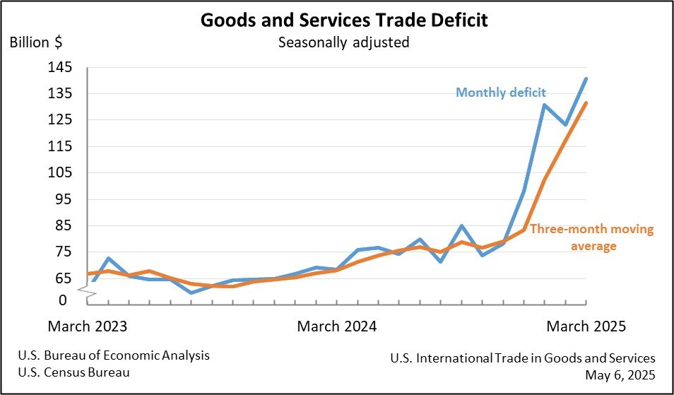
Chart IIA-1A of the US Census Bureau of the Department of Commerce shows that the trade deficit (gap between exports and imports) fell during the economic contraction after 2007 but has grown again during the expansion. The low average rate of growth of GDP of 2.2 percent during the expansion beginning since IIIQ2009 does not deteriorate further the trade balance. Higher rates of growth may cause sharper deterioration.
Chart IIA-1, US, International Trade Balance, Exports and Imports of Goods and Services USD Billions
Source: US Census Bureau
https://www.census.gov/foreign-trade/data/ustrade.jpg
Table IIA-2B provides the US international trade balance, exports and imports of goods and services on an annual basis from 1992 to 2017. The trade balance deteriorated sharply over the long term. The US has a large deficit in goods or exports less imports of goods but it has a surplus in services that helps to reduce the trade account deficit or exports less imports of goods and services. The current account deficit of the US not seasonally adjusted increased from $84.8 billion in IQ2017 to $96.9 billion in IQ2018 (https://www.bea.gov/international/index.htm). The current account deficit seasonally adjusted at annual rate increased from 2.3 percent of GDP in IQ2017 to 2.4 percent of GDP in IVQ2017, increasing to 2.5 percent of GDP in IQ2018. The ratio of the current account deficit to GDP has stabilized below 3 percent of GDP compared with much higher percentages before the recession but is combined now with much higher imbalance in the Treasury budget (see Pelaez and Pelaez, The Global Recession Risk (2007), Globalization and the State, Vol. II (2008b), 183-94, Government Intervention in Globalization (2008c), 167-71). There is still a major challenge in the combined deficits in current account and in federal budgets. The final rows of Table IIA-2B show marginal improvement of the trade deficit from $549,699 million in 2011 to lower $537,408 million in 2012 with exports growing 4.3 percent and imports 3.0 percent. The trade balance improved further to deficit of $461,135 million in 2013 with growth of exports of 3.4 percent while imports virtually stagnated. The trade deficit deteriorated in 2014 to $489,584 million with growth of exports of 3.6 percent and of imports of 4.0 percent. The trade deficit deteriorated in 2015 to $498,525 million with decrease of exports of 4.6 percent and decrease of imports of 3.5 percent. The trade deficit deteriorated in 2016 to $502.001 million with decrease of exports of 2.2 percent and decrease of imports of 1.7 percent. The trade deficit deteriorated in 2017 to $552,277 million with growth of exports of 6.1 percent and of imports of 6.8 percent. Growth and commodity shocks under alternating inflation waves (https://cmpassocregulationblog.blogspot.com/2018/06/world-inflation-waves-united-states.html) have deteriorated the trade deficit from the low of $383,774 million in 2009.
Table IIA-2B, US, International Trade Balance of Goods and Services, Exports and Imports of Goods and Services, SA, Millions of Dollars, Balance of Payments Basis
| Balance | Exports | ∆% | Imports | ∆% | |
| 1960 | 3,508 | 25,940 | 22,432 | ||
| 1961 | 4,195 | 26,403 | 1.8 | 22,208 | -1.0 |
| 1962 | 3,370 | 27,722 | 5.0 | 24,352 | 9.7 |
| 1963 | 4,210 | 29,620 | 6.8 | 25,410 | 4.3 |
| 1964 | 6,022 | 33,341 | 12.6 | 27,319 | 7.5 |
| 1965 | 4,664 | 35,285 | 5.8 | 30,621 | 12.1 |
| 1966 | 2,939 | 38,926 | 10.3 | 35,987 | 17.5 |
| 1967 | 2,604 | 41,333 | 6.2 | 38,729 | 7.6 |
| 1968 | 250 | 45,543 | 10.2 | 45,293 | 16.9 |
| 1969 | 91 | 49,220 | 8.1 | 49,129 | 8.5 |
| 1970 | 2,254 | 56,640 | 15.1 | 54,386 | 10.7 |
| 1971 | -1,302 | 59,677 | 5.4 | 60,979 | 12.1 |
| 1972 | -5,443 | 67,222 | 12.6 | 72,665 | 19.2 |
| 1973 | 1,900 | 91,242 | 35.7 | 89,342 | 23.0 |
| 1974 | -4,293 | 120,897 | 32.5 | 125,190 | 40.1 |
| 1975 | 12,404 | 132,585 | 9.7 | 120,181 | -4.0 |
| 1976 | -6,082 | 142,716 | 7.6 | 148,798 | 23.8 |
| 1977 | -27,246 | 152,301 | 6.7 | 179,547 | 20.7 |
| 1978 | -29,763 | 178,428 | 17.2 | 208,191 | 16.0 |
| 1979 | -24,565 | 224,131 | 25.6 | 248,696 | 19.5 |
| 1980 | -19,407 | 271,834 | 21.3 | 291,241 | 17.1 |
| 1981 | -16,172 | 294,398 | 8.3 | 310,570 | 6.6 |
| 1982 | -24,156 | 275,236 | -6.5 | 299,391 | -3.6 |
| 1983 | -57,767 | 266,106 | -3.3 | 323,874 | 8.2 |
| 1984 | -109,072 | 291,094 | 9.4 | 400,166 | 23.6 |
| 1985 | -121,880 | 289,070 | -0.7 | 410,950 | 2.7 |
| 1986 | -138,538 | 310,033 | 7.3 | 448,572 | 9.2 |
| 1987 | -151,684 | 348,869 | 12.5 | 500,552 | 11.6 |
| 1988 | -114,566 | 431,149 | 23.6 | 545,715 | 9.0 |
| 1989 | -93,141 | 487,003 | 13.0 | 580,144 | 6.3 |
| 1990 | -80,864 | 535,233 | 9.9 | 616,097 | 6.2 |
| 1991 | -31,135 | 578,344 | 8.1 | 609,479 | -1.1 |
| 1992 | -39,212 | 616,882 | 6.7 | 656,094 | 7.6 |
| 1993 | -70,311 | 642,863 | 4.2 | 713,174 | 8.7 |
| 1994 | -98,493 | 703,254 | 9.4 | 801,747 | 12.4 |
| 1995 | -96,384 | 794,387 | 13.0 | 890,771 | 11.1 |
| 1996 | -104,065 | 851,602 | 7.2 | 955,667 | 7.3 |
| 1997 | -108,273 | 934,453 | 9.7 | 1,042,726 | 9.1 |
| 1998 | -166,140 | 933,174 | -0.1 | 1,099,314 | 5.4 |
| 1999 | -258,617 | 969,867 | 3.9 | 1,228,485 | 11.8 |
| 2000 | -372,517 | 1,075,321 | 10.9 | 1,447,837 | 17.9 |
| 2001 | -361,511 | 1,005,654 | -6.5 | 1,367,165 | -5.6 |
| 2002 | -418,955 | 978,706 | -2.7 | 1,397,660 | 2.2 |
| 2003 | -493,890 | 1,020,418 | 4.3 | 1,514,308 | 8.3 |
| 2004 | -609,883 | 1,161,549 | 13.8 | 1,771,433 | 17.0 |
| 2005 | -714,245 | 1,286,022 | 10.7 | 2,000,267 | 12.9 |
| 2006 | -761,716 | 1,457,642 | 13.3 | 2,219,358 | 11.0 |
| 2007 | -705,375 | 1,653,548 | 13.4 | 2,358,922 | 6.3 |
| 2008 | -708,726 | 1,841,612 | 11.4 | 2,550,339 | 8.1 |
| 2009 | -383,774 | 1,583,053 | -14.0 | 1,966,827 | -22.9 |
| 2010 | -495,225 | 1,853,038 | 17.1 | 2,348,263 | 19.4 |
| 2011 | -549,699 | 2,125,947 | 14.7 | 2,675,646 | 13.9 |
| 2012 | -537,408 | 2,218,354 | 4.3 | 2,755,762 | 3.0 |
| 2013 | -461,135 | 2,294,199 | 3.4 | 2,755,334 | 0.0 |
| 2014 | -489,584 | 2,376,657 | 3.6 | 2,866,241 | 4.0 |
| 2015 | -498,525 | 2,266,691 | -4.6 | 2,765,216 | -3.5 |
| 2016 | -502,001 | 2,215,844 | -2.2 | 2,717,846 | -1.7 |
| 2017 | -552,277 | 2,351,072 | 6.1 | 2,903,349 | 6.8 |
Source: US Census Bureau
http://www.census.gov/foreign-trade/
Chart IIA-2 of the US Census Bureau provides the US trade account in goods and services SA from Jan 1992 to May 2018. There is long-term trend of deterioration of the US trade deficit shown vividly by Chart IIA-2. The global recession from IVQ2007 to IIQ2009 reversed the trend of deterioration. Deterioration resumed together with incomplete recovery and was influenced significantly by the carry trade from zero interest rates to commodity futures exposures (these arguments are elaborated in Pelaez and Pelaez, Financial Regulation after the Global Recession (2009a), 157-66, Regulation of Banks and Finance (2009b), 217-27, International Financial Architecture (2005), 15-18, The Global Recession Risk (2007), 221-5, Globalization and the State Vol. II (2008b), 197-213, Government Intervention in Globalization (2008c), 182-4 http://cmpassocregulationblog.blogspot.com/2011/07/causes-of-2007-creditdollar-crisis.html http://cmpassocregulationblog.blogspot.com/2011/01/professor-mckinnons-bubble-economy.html http://cmpassocregulationblog.blogspot.com/2011/01/world-inflation-quantitative-easing.html http://cmpassocregulationblog.blogspot.com/2011/01/treasury-yields-valuation-of-risk.html http://cmpassocregulationblog.blogspot.com/2010/11/quantitative-easing-theory-evidence-and.html http://cmpassocregulationblog.blogspot.com/2010/12/is-fed-printing-money-what-are.html). Earlier research focused on the long-term external imbalance of the US in the form of trade and current account deficits (Pelaez and Pelaez, The Global Recession Risk (2007), Globalization and the State Vol. II (2008b) 183-94, Government Intervention in Globalization (2008c), 167-71). US external imbalances have not been fully resolved and tend to widen together with improving world economic activity and commodity price shocks. There are additional effects for revaluation of the dollar with the Fed orienting interest rate increases while the European Central Bank and the Bank of Japan determine negative nominal interest rates.
Chart IIA-2, US, Balance of Trade SA, Monthly, Millions of Dollars, Jan 1992-May 2018
Source: US Census Bureau
http://www.census.gov/foreign-trade/
Chart IIA-3 of the US Census Bureau provides US exports SA from Jan 1992 to May 2018. There was sharp acceleration from 2003 to 2007 during worldwide economic boom and increasing inflation. Exports fell sharply during the financial crisis and global recession from IVQ2007 to IIQ2009. Growth picked up again together with world trade and inflation but stalled in the final segment with less rapid global growth and inflation.
Chart IIA-3, US, Exports SA, Monthly, Millions of Dollars Jan 1992-May 2018
Source: US Census Bureau
http://www.census.gov/foreign-trade/
Chart IIA-4 of the US Census Bureau provides US imports SA from Jan 1992 to May 2018. Growth was stronger between 2003 and 2007 with worldwide economic boom and inflation. There was sharp drop during the financial crisis and global recession. There is stalling import levels in the final segment resulting from weaker world economic growth and diminishing inflation because of risk aversion and portfolio reallocations from commodity exposures to equities.
Chart IIA-4, US, Imports SA, Monthly, Millions of Dollars Jan 1992-May 2018
Source: US Census Bureau
http://www.census.gov/foreign-trade/
There is improvement of the US trade balance in goods in Table IIA-3 from deficit of $66,768 million in May 2017 to deficit of $65,787 million in May 2018. The nonpetroleum deficit increased $186 million while the petroleum deficit decreased $1131 million. Total exports of goods increased 14.0 percent in May 2018 relative to a year earlier while total imports increased 8.7 percent. Nonpetroleum exports increased 11.2 percent from May 2017 to May 2018 while nonpetroleum imports increased 7.5 percent. Petroleum imports increased 21.5 percent.
Table IIA-3, US, International Trade in Goods Balance, Exports and Imports $ Millions and ∆% SA
| May 2018 | May 2017 | ∆% | |
| Total Balance | -65,787 | -66,768 | |
| Petroleum | -4,624 | -5,755 | |
| Non-Petroleum | -60,143 | -59,954 | |
| Total Exports | 144,888 | 127,091 | 14.0 |
| Petroleum | 14,179 | 9,720 | 45.9 |
| Non-Petroleum | 129,976 | 116,848 | 11.2 |
| Total Imports | 210,675 | 193,859 | 8.7 |
| Petroleum | 18,803 | 15,474 | 21.5 |
| Non-Petroleum | 190,119 | 176,803 | 7.5 |
Details may not add because of rounding and seasonal adjustment
Source: US Census Bureau
http://www.census.gov/foreign-trade/
US exports and imports of goods not seasonally adjusted in Jan-May 2018 and Jan-May 2017 are in Table IIA-4. The rate of growth of exports was 9.7 percent and 9.1 percent for imports. The US has partial hedge of commodity price increases in exports of agricultural commodities that increased 4.3 percent and of mineral fuels that increased 33.8 percent both because prices of raw materials and commodities increase and fall recurrently because of shocks of risk aversion and portfolio reallocations. The US exports a growing amount of crude oil, increasing 39.1 percent in cumulative Jan-May 2018 relative to a year earlier. US exports and imports consist mostly of manufactured products, with less rapidly increasing prices. US manufactured exports increased 7.4 percent while manufactured imports increased 9.4 percent. Significant part of the US trade imbalance originates in imports of mineral fuels increasing 12.7 percent and petroleum increasing 14.3 percent with wide oscillations in oil prices. The limited hedge in exports of agricultural commodities and mineral fuels compared with substantial imports of mineral fuels and crude oil results in waves of deterioration of the terms of trade of the US, or export prices relative to import prices, originating in commodity price increases caused by carry trades from zero interest rates. These waves are similar to those in worldwide inflation.
Table IIA-4, US, Exports and Imports of Goods, Not Seasonally Adjusted Millions of Dollars and %, Census Basis
| Jan-May 2018 $ Millions | Jan-May 2017 $ Millions | ∆% | |
| Exports | 684,626 | 624,238 | 9.7 |
| Manufactured | 478,728 | 445,839 | 7.4 |
| Agricultural | 59,792 | 57,332 | 4.3 |
| Mineral Fuels | 71,004 | 53,087 | 33.8 |
| Petroleum | 54,844 | 39,419 | 39.1 |
| Imports | 1,021,168 | 936,069 | 9.1 |
| Manufactured | 876,208 | 801,067 | 9.4 |
| Agricultural | 56,162 | 51,324 | 9.4 |
| Mineral Fuels | 92,855 | 82,414 | 12.7 |
| Petroleum | 87,488 | 76,565 | 14.3 |
Source: US Census Bureau
http://www.census.gov/foreign-trade/
The current account of the US balance of payments is in Table VI-3A for IQ2017 and IQ2018. The Bureau of Economic Analysis analyzes as follows (https://www.bea.gov/newsreleases/international/transactions/2018/pdf/trans118.pdf):
“The U.S. current-account deficit increased to $124.1 billion (preliminary) in the first quarter of 2018 from $116.1 billion (revised) in the fourth quarter of 2017, according to statistics released by the Bureau of Economic Analysis (BEA). The deficit was 2.5 percent of current-dollar gross domestic product (GDP) in the first quarter, up from 2.4 percent in the fourth quarter.”
The US has a large deficit in goods or exports less imports of goods but it has a surplus in services that helps to reduce the trade account deficit or exports less imports of goods and services. The current account deficit of the US not seasonally adjusted increased from $84.8 billion in IQ2017 to $96.9 billion in IQ2018. The current account deficit seasonally adjusted at annual rate increased from 2.3 percent of GDP in IQ2017 to 2.4 percent of GDP in IVQ2017, increasing to 2.5 percent of GDP in IQ2018. The ratio of the current account deficit to GDP has stabilized below 3 percent of GDP compared with much higher percentages before the recession but is combined now with much higher imbalance in the Treasury budget (see Pelaez and Pelaez, The Global Recession Risk (2007), Globalization and the State, Vol. II (2008b), 183-94, Government Intervention in Globalization (2008c), 167-71). There is still a major challenge in the combined deficits in current account and in federal budgets.
Table VI-3A, US, Balance of Payments, Millions of Dollars NSA
| IQ2017 | IQ2018 | Difference | |
| Goods Balance | -180,110 | -199,502 | -19,392 |
| X Goods | 374,213 | 404,253 | 8.0 ∆% |
| M Goods | -554,323 | -603,755 | 8.9 ∆% |
| Services Balance | 68,748 | 71,526 | 2,778 |
| X Services | 193,251 | 206,844 | 7.0 ∆% |
| M Services | -124,503 | -135,318 | 7.9 ∆% |
| Balance Goods and Services | -111,362 | -127,976 | -16,614 |
| Exports of Goods and Services and Income Receipts | 822,466 | 901,459 | |
| Imports of Goods and Services and Income Payments | -907,305 | -998,319 | |
| Current Account Balance | -84,839 | -96,860 | -12,021 |
| % GDP | IQ2017 | IQ2018 | IVQ2017 |
| 2.3 | 2.5 | 2.4 |
X: exports; M: imports
Balance on Current Account = Exports of Goods and Services – Imports of Goods and Services and Income Payments
Source: Bureau of Economic Analysis
http://www.bea.gov/international/index.htm#bop
In their classic work on “unpleasant monetarist arithmetic,” Sargent and Wallace (1981, 2) consider a regime of domination of monetary policy by fiscal policy (emphasis added):
“Imagine that fiscal policy dominates monetary policy. The fiscal authority independently sets its budgets, announcing all current and future deficits and surpluses and thus determining the amount of revenue that must be raised through bond sales and seignorage. Under this second coordination scheme, the monetary authority faces the constraints imposed by the demand for government bonds, for it must try to finance with seignorage any discrepancy between the revenue demanded by the fiscal authority and the amount of bonds that can be sold to the public. Suppose that the demand for government bonds implies an interest rate on bonds greater than the economy’s rate of growth. Then if the fiscal authority runs deficits, the monetary authority is unable to control either the growth rate of the monetary base or inflation forever. If the principal and interest due on these additional bonds are raised by selling still more bonds, so as to continue to hold down the growth of base money, then, because the interest rate on bonds is greater than the economy’s growth rate, the real stock of bonds will growth faster than the size of the economy. This cannot go on forever, since the demand for bonds places an upper limit on the stock of bonds relative to the size of the economy. Once that limit is reached, the principal and interest due on the bonds already sold to fight inflation must be financed, at least in part, by seignorage, requiring the creation of additional base money.”
The alternative fiscal scenario of the CBO (2012NovCDR, 2013Sep17) resembles an economic world in which eventually the placement of debt reaches a limit of what is proportionately desired of US debt in investment portfolios. This unpleasant environment is occurring in various European countries.
The current real value of government debt plus monetary liabilities depends on the expected discounted values of future primary surpluses or difference between tax revenue and government expenditure excluding interest payments (Cochrane 2011Jan, 27, equation (16)). There is a point when adverse expectations about the capacity of the government to generate primary surpluses to honor its obligations can result in increases in interest rates on government debt.
First, Unpleasant Monetarist Arithmetic. Fiscal policy is described by Sargent and Wallace (1981, 3, equation 1) as a time sequence of D(t), t = 1, 2,…t, …, where D is real government expenditures, excluding interest on government debt, less real tax receipts. D(t) is the real deficit excluding real interest payments measured in real time t goods. Monetary policy is described by a time sequence of H(t), t=1,2,…t, …, with H(t) being the stock of base money at time t. In order to simplify analysis, all government debt is considered as being only for one time period, in the form of a one-period bond B(t), issued at time t-1 and maturing at time t. Denote by R(t-1) the real rate of interest on the one-period bond B(t) between t-1 and t. The measurement of B(t-1) is in terms of t-1 goods and [1+R(t-1)] “is measured in time t goods per unit of time t-1 goods” (Sargent and Wallace 1981, 3). Thus, B(t-1)[1+R(t-1)] brings B(t-1) to maturing time t. B(t) represents borrowing by the government from the private sector from t to t+1 in terms of time t goods. The price level at t is denoted by p(t). The budget constraint of Sargent and Wallace (1981, 3, equation 1) is:
D(t) = {[H(t) – H(t-1)]/p(t)} + {B(t) – B(t-1)[1 + R(t-1)]} (1)
Equation (1) states that the government finances its real deficits into two portions. The first portion, {[H(t) – H(t-1)]/p(t)}, is seigniorage, or “printing money.” The second part,
{B(t) – B(t-1)[1 + R(t-1)]}, is borrowing from the public by issue of interest-bearing securities. Denote population at time t by N(t) and growing by assumption at the constant rate of n, such that:
N(t+1) = (1+n)N(t), n>-1 (2)
The per capita form of the budget constraint is obtained by dividing (1) by N(t) and rearranging:
B(t)/N(t) = {[1+R(t-1)]/(1+n)}x[B(t-1)/N(t-1)]+[D(t)/N(t)] – {[H(t)-H(t-1)]/[N(t)p(t)]} (3)
On the basis of the assumptions of equal constant rate of growth of population and real income, n, constant real rate of return on government securities exceeding growth of economic activity and quantity theory equation of demand for base money, Sargent and Wallace (1981) find that “tighter current monetary policy implies higher future inflation” under fiscal policy dominance of monetary policy. That is, the monetary authority does not permanently influence inflation, lowering inflation now with tighter policy but experiencing higher inflation in the future.
Second, Unpleasant Fiscal Arithmetic. The tool of analysis of Cochrane (2011Jan, 27, equation (16)) is the government debt valuation equation:
(Mt + Bt)/Pt = Et∫(1/Rt, t+τ)st+τdτ (4)
Equation (4) expresses the monetary, Mt, and debt, Bt, liabilities of the government, divided by the price level, Pt, in terms of the expected value discounted by the ex-post rate on government debt, Rt, t+τ, of the future primary surpluses st+τ, which are equal to Tt+τ – Gt+τ or difference between taxes, T, and government expenditures, G. Cochrane (2010A) provides the link to a web appendix demonstrating that it is possible to discount by the ex post Rt, t+τ. The second equation of Cochrane (2011Jan, 5) is:
MtV(it, ·) = PtYt (5)
Conventional analysis of monetary policy contends that fiscal authorities simply adjust primary surpluses, s, to sanction the price level determined by the monetary authority through equation (5), which deprives the debt valuation equation (4) of any role in price level determination. The simple explanation is (Cochrane 2011Jan, 5):
“We are here to think about what happens when [4] exerts more force on the price level. This change may happen by force, when debt, deficits and distorting taxes become large so the Treasury is unable or refuses to follow. Then [4] determines the price level; monetary policy must follow the fiscal lead and ‘passively’ adjust M to satisfy [5]. This change may also happen by choice; monetary policies may be deliberately passive, in which case there is nothing for the Treasury to follow and [4] determines the price level.”
An intuitive interpretation by Cochrane (2011Jan 4) is that when the current real value of government debt exceeds expected future surpluses, economic agents unload government debt to purchase private assets and goods, resulting in inflation. If the risk premium on government debt declines, government debt becomes more valuable, causing a deflationary effect. If the risk premium on government debt increases, government debt becomes less valuable, causing an inflationary effect.
There are multiple conclusions by Cochrane (2011Jan) on the debt/dollar crisis and Global recession, among which the following three:
(1) The flight to quality that magnified the recession was not from goods into money but from private-sector securities into government debt because of the risk premium on private-sector securities; monetary policy consisted of providing liquidity in private-sector markets suffering stress
(2) Increases in liquidity by open-market operations with short-term securities have no impact; quantitative easing can affect the timing but not the rate of inflation; and purchase of private debt can reverse part of the flight to quality
(3) The debt valuation equation has a similar role as the expectation shifting the Phillips curve such that a fiscal inflation can generate stagflation effects similar to those occurring from a loss of anchoring expectations.
This analysis suggests that there may be a point of saturation of demand for United States financial liabilities without an increase in interest rates on Treasury securities. A risk premium may develop on US debt. Such premium is not apparent currently because of distressed conditions in the world economy and international financial system. Risk premiums are observed in the spread of bonds of highly indebted countries in Europe relative to bonds of the government of Germany.
The issue of global imbalances centered on the possibility of a disorderly correction (Pelaez and Pelaez, The Global Recession Risk (2007), Globalization and the State Vol. II (2008b) 183-94, Government Intervention in Globalization (2008c), 167-71). Such a correction has not occurred historically but there is no argument proving that it could not occur. The need for a correction would originate in unsustainable large and growing United States current account deficits (CAD) and net international investment position (NIIP) or excess of financial liabilities of the US held by foreigners net relative to financial liabilities of foreigners held by US residents. The IMF estimated that the US could maintain a CAD of two to three percent of GDP without major problems (Rajan 2004). The threat of disorderly correction is summarized by Pelaez and Pelaez, The Global Recession Risk (2007), 15):
“It is possible that foreigners may be unwilling to increase their positions in US financial assets at prevailing interest rates. An exit out of the dollar could cause major devaluation of the dollar. The depreciation of the dollar would cause inflation in the US, leading to increases in American interest rates. There would be an increase in mortgage rates followed by deterioration of real estate values. The IMF has simulated that such an adjustment would cause a decline in the rate of growth of US GDP to 0.5 percent over several years. The decline of demand in the US by four percentage points over several years would result in a world recession because the weakness in Europe and Japan could not compensate for the collapse of American demand. The probability of occurrence of an abrupt adjustment is unknown. However, the adverse effects are quite high, at least hypothetically, to warrant concern.”
The United States could be moving toward a situation typical of heavily indebted countries, requiring fiscal adjustment and increases in productivity to become more competitive internationally. The CAD and NIIP of the United States are not observed in full deterioration because the economy is well below trend. There are two complications in the current environment relative to the concern with disorderly correction in the first half of the past decade. In the release of Jun 14, 2013, the Bureau of Economic Analysis (http://www.bea.gov/newsreleases/international/transactions/2013/pdf/trans113.pdf) informs of revisions of US data on US international transactions since 1999:
“The statistics of the U.S. international transactions accounts released today have been revised for the first quarter of 1999 to the fourth quarter of 2012 to incorporate newly available and revised source data, updated seasonal adjustments, changes in definitions and classifications, and improved estimating methodologies.”
The BEA introduced new concepts and methods (http://www.bea.gov/international/concepts_methods.htm) in comprehensive restructuring on Jun 18, 2014 (http://www.bea.gov/international/modern.htm):
“BEA introduced a new presentation of the International Transactions Accounts on June 18, 2014 and will introduce a new presentation of the International Investment Position on June 30, 2014. These new presentations reflect a comprehensive restructuring of the international accounts that enhances the quality and usefulness of the accounts for customers and bring the accounts into closer alignment with international guidelines.”
Table VI-3B provides data on the US fiscal and balance of payments imbalances incorporating all revisions and methods. In 2007, the federal deficit of the US was $161 billion corresponding to 1.1 percent of GDP while the Congressional Budget Office estimates the federal deficit in 2012 at $1087 billion or 6.8 percent of GDP. The estimate of the deficit for 2013 is $680 billion or 4.1 percent of GDP. The combined record federal deficits of the US from 2009 to 2012 are $5094 billion or 31.6 percent of the estimate of GDP for fiscal year 2012 implicit in the CBO (CBO 2013Sep11) estimate of debt/GDP. The deficits from 2009 to 2012 exceed one trillion dollars per year, adding to $5.094 trillion in four years, using the fiscal year deficit of $1087 billion for fiscal year 2012, which is the worst fiscal performance since World War II. Federal debt in 2007 was $5035 billion, slightly less than the combined deficits from 2009 to 2012 of $5094 billion. Federal debt in 2012 was 70.4 percent of GDP (CBO 2015Jan26) and 72.6 percent of GDP in 2013 (http://www.cbo.gov/). This situation may worsen in the future (CBO 2013Sep17):
“Between 2009 and 2012, the federal government recorded the largest budget deficits relative to the size of the economy since 1946, causing federal debt to soar. Federal debt held by the public is now about 73 percent of the economy’s annual output, or gross domestic product (GDP). That percentage is higher than at any point in U.S. history except a brief period around World War II, and it is twice the percentage at the end of 2007. If current laws generally remained in place, federal debt held by the public would decline slightly relative to GDP over the next several years, CBO projects. After that, however, growing deficits would ultimately push debt back above its current high level. CBO projects that federal debt held by the public would reach 100 percent of GDP in 2038, 25 years from now, even without accounting for the harmful effects that growing debt would have on the economy. Moreover, debt would be on an upward path relative to the size of the economy, a trend that could not be sustained indefinitely.
The gap between federal spending and revenues would widen steadily after 2015 under the assumptions of the extended baseline, CBO projects. By 2038, the deficit would be 6½ percent of GDP, larger than in any year between 1947 and 2008, and federal debt held by the public would reach 100 percent of GDP, more than in any year except 1945 and 1946. With such large deficits, federal debt would be growing faster than GDP, a path that would ultimately be unsustainable.
Incorporating the economic effects of the federal policies that underlie the extended baseline worsens the long-term budget outlook. The increase in debt relative to the size of the economy, combined with an increase in marginal tax rates (the rates that would apply to an additional dollar of income), would reduce output and raise interest rates relative to the benchmark economic projections that CBO used in producing the extended baseline. Those economic differences would lead to lower federal revenues and higher interest payments. With those effects included, debt under the extended baseline would rise to 108 percent of GDP in 2038.”
The CBO long-term budget on Mar 27, 2017, projects US federal debt at 150.0 percent of GDP in 2047 (Congressional Budget Office, The 2017 Long-term Budget Outlook. Washington, DC, Mar 30, 2017 https://www.cbo.gov/publication/52480).
Table VI-3B, US, Current Account, NIIP, Fiscal Balance, Nominal GDP, Federal Debt and Direct Investment, Dollar Billions and %
| 2007 | 2008 | 2009 | 2010 | 2011 | |
| Goods & | -705 | -709 | -384 | -495 | -549 |
| Primary Income | 85 | 130 | 115 | 168 | 211 |
| Secondary Income | -91 | -102 | -104 | -104 | -107 |
| Current Account | -711 | -681 | -373 | -431 | -445 |
| NGDP | 14478 | 14719 | 14419 | 14964 | 15518 |
| Current Account % GDP | -4.9 | -4.6 | -2.6 | -2.9 | -2.9 |
| NIIP | -1279 | -3995 | -2628 | -2512 | -4455 |
| US Owned Assets Abroad | 20705 | 19423 | 19426 | 21767 | 22209 |
| Foreign Owned Assets in US | 21984 | 23418 | 22054 | 24279 | 26664 |
| NIIP % GDP | -8.8 | -27.1 | -18.2 | -16.8 | -28.7 |
| Exports | 2559 | 2742 | 2283 | 2625 | 2983 |
| NIIP % | -50 | -145 | -115 | -95 | -149 |
| DIA MV | 5858 | 3707 | 4945 | 5486 | 5215 |
| DIUS MV | 4134 | 3091 | 3619 | 4099 | 4199 |
| Fiscal Balance | -161 | -459 | -1413 | -1294 | -1300 |
| Fiscal Balance % GDP | -1.1 | -3.1 | -9.8 | -8.7 | -8.5 |
| Federal Debt | 5035 | 5803 | 7545 | 9019 | 10128 |
| Federal Debt % GDP | 35.2 | 39.3 | 52.3 | 60.9 | 65.9 |
| Federal Outlays | 2729 | 2983 | 3518 | 3457 | 3603 |
| ∆% | 2.8 | 9.3 | 17.9 | -1.7 | 4.2 |
| % GDP | 19.1 | 20.2 | 24.4 | 23.4 | 23.4 |
| Federal Revenue | 2568 | 2524 | 2105 | 2163 | 2303 |
| ∆% | 6.7 | -1.7 | -16.6 | 2.7 | 6.5 |
| % GDP | 17.9 | 17.1 | 14.6 | 14.6 | 15.0 |
| 2012 | 2013 | 2014 | 2015 | 2016 | |
| Goods & | -537 | -462 | -490 | -500 | -505 |
| Primary Income | 207 | 206 | 210 | 181 | 173 |
| Secondary Income | -97 | -94 | -94 | -115 | -120 |
| Current Account | -426 | -350 | -374 | -434 | -452 |
| NGDP | 16155 | 16692 | 17428 | 18121 | 18625 |
| Current Account % GDP | -2.6 | -2.1 | -2.1 | -2.4 | -2.4 |
| NIIP | -4518 | -5373 | -6980 | -7493 | -8318 |
| US Owned Assets Abroad | 22562 | 24145 | 24832 | 23352 | 23849 |
| Foreign Owned Assets in US | 27080 | 29517 | 31813 | 30846 | 32168 |
| NIIP % GDP | -28.0 | -32.2 | -40.1 | -41.3 | -44.7 |
| Exports | 3096 | 3212 | 3333 | 3173 | 3157 |
| NIIP % | -146 | -167 | -209 | -236 | -263 |
| DIA MV | 5969 | 7121 | 7189 | 6999 | 7375 |
| DIUS MV | 4662 | 5815 | 6370 | 6701 | 7569 |
| Fiscal Balance | -1087 | -680 | -485 | -439 | -585 |
| Fiscal Balance % GDP | -6.8 | -4.1 | -2.8 | -2.4 | -3.2 |
| Federal Debt | 11281 | 11983 | 12780 | 13117 | 14168 |
| Federal Debt % GDP | 70.4 | 72.6 | 74.2 | 73.3 | 77.0 |
| Federal Outlays | 3537 | 3455 | 3506 | 3688 | 3853 |
| ∆% | -1.8 | -2.3 | 1.5 | 5.2 | 4.5 |
| % GDP | 22.1 | 20.9 | 20.4 | 20.6 | 20.9 |
| Federal Revenue | 2450 | 2775 | 3022 | 3250 | 3268 |
| ∆% | 6.4 | 13.3 | 8.9 | 7.6 | 0.5 |
| % GDP | 15.3 | 16.8 | 17.5 | 18.2 | 17.8 |
Sources:
Notes: NGDP: nominal GDP or in current dollars; NIIP: Net International Investment Position; DIA MV: US Direct Investment Abroad at Market Value; DIUS MV: Direct Investment in the US at Market Value. There are minor discrepancies in the decimal point of percentages of GDP between the balance of payments data and federal debt, outlays, revenue and deficits in which the original number of the CBO source is maintained. See Bureau of Economic Analysis, US International Economic Accounts: Concepts and Methods. 2014. Washington, DC: BEA, Department of Commerce, Jun 2014 http://www.bea.gov/international/concepts_methods.htm These discrepancies do not alter conclusions. Budget http://www.cbo.gov/
https://www.cbo.gov/about/products/budget-economic-data#6
https://www.cbo.gov/about/products/budget_economic_data#3
https://www.cbo.gov/about/products/budget-economic-data#2
https://www.cbo.gov/about/products/budget_economic_data#2 Balance of Payments and NIIP http://www.bea.gov/international/index.htm#bop Gross Domestic Product, Bureau of Economic Analysis (BEA) http://www.bea.gov/iTable/index_nipa.cfm
Table VI-3C provides quarterly estimates NSA of the external imbalance of the United States. The current account deficit seasonally adjusted at 2.3 percent of GDP in IQ2017 deteriorates to 2.5 percent in IIQ2017. The current account deficit decreased to 2.1 percent in IIIQ2017. The current account deficit increased to 2.4 percent in IVQ2017. The current account deficit increases to 2.5 percent in IQ2018. The absolute value of the net international investment position decreases from minus $8.0 trillion in IQ2017 to minus $7.9 trillion in IIQ2017. The absolute value of the net international investment position decreased to $7.6 trillion in IIIQ2017. The absolute value of the net international investment position stabilizes at $7.7 trillion in IVQ2017. The absolute value of the net international investment position deteriorates to $7.9 trillion in IQ2018. The BEA explains as follows (https://www.bea.gov/newsreleases/international/intinv/2018/pdf/intinv118.pdf):
“The U.S. net international investment position decreased to −$7,888.1 billion (preliminary) at the end of the first quarter of 2018 from −$7,725.0 billion (revised) at the end of the fourth quarter of 2017, according to statistics released by the Bureau of Economic Analysis (BEA). The $163.1 billion decrease reflected a $182.8 billion decrease in U.S. assets and a $19.7 billion decrease in U.S. liabilities (table 1).”
The BEA explains further (https://www.bea.gov/newsreleases/international/intinv/2018/pdf/intinv118.pdf):
“The $163.1 billion decrease in the net investment position reflected net financial transactions of –$164.8 billion and net other changes in position, such as price and exchange-rate changes, of $1.7 billion (table A). The net investment position decreased 2.1 percent in the first quarter, compared with a decrease of 1.3 percent in the fourth quarter. The net investment position decreased an average of 4.7 percent from the first quarter of 2011 through the third quarter of 2017.
U.S. assets decreased $182.8 billion to $27,616.3 billion at the end of the first quarter, mostly reflecting a decrease in direct investment assets that was partly offset by an increase in portfolio investment assets.
• Assets excluding financial derivatives decreased $171.9 billion to $26,004.7 billion. The decrease resulted from other changes in position of –$440.8 billion and financial transactions of $268.9 billion (table A).
o Other changes in position were driven by foreign equity price decreases that lowered the value of portfolio investment and direct investment equity assets. These price decreases were partly offset by increases from exchange-rate changes, as major foreign currencies appreciated against the U.S. dollar, raising the value of foreign-currency denominated assets in dollar terms.
o Financial transactions mostly reflected net acquisition of portfolio investment assets that was partly offset by net withdrawal of direct investment assets. The net withdrawal of direct investment assets resulted from U.S. parent repatriation of previously reinvested earnings. For more information on the repatriation, see the box Effects of the 2017 Tax Cuts and Jobs Act on Components of Direct Investment.’
• Financial derivatives decreased $10.9 billion to $1,611.6 billion, reflecting decreases in single currency interest rate contracts and foreign exchange contracts.”
| IQ2017 | IIQ2017 | IIIQ2017 | IVQ2017 | IQ2018 | |
| Goods & | -111 | -150 | -142 | -149 | -128 |
| Primary Income | 53 | 48 | 58 | 63 | 62 |
| Secondary Income | -26 | -32 | -30 | -30 | -31 |
| Current Account | -84 | -134 | -114 | -116 | -97 |
| Current Account % GDP SA | -2.3 | -2.5 | -2.1 | -2.4 | -2.5 |
| NIIP | -7986 | -7858 | -7625 | -7725 | -7888 |
| US Owned Assets Abroad | 25118 | 26083 | 27124 | 27799 | 27616 |
| Foreign Owned Assets in US | -33104 | -33941 | -34749 | -35524 | -35504 |
| DIA MV | 7921 | 8183 | 8657 | 8910 | 8542 |
| DIA MV Equity | 6637 | 6941 | 7381 | 7646 | 7232 |
| DIUS MV | 7992 | 8207 | 8531 | 8925 | 8872 |
| DIUS MV Equity | 6629 | 6424 | 6714 | 7133 | 7059 |
Notes: NIIP: Net International Investment Position; DIA MV: US Direct Investment Abroad at Market Value; DIUS MV: Direct Investment in the US at Market Value. See Bureau of Economic Analysis, US International Economic Accounts: Concepts and Methods. 2014. Washington, DC: BEA, Department of Commerce, Jun 2014 http://www.bea.gov/international/concepts_methods.htm
Chart VI-3C of the US Bureau of Economic Analysis provides the quarterly and annual US net international investment position (NIIP) NSA in billion dollars. The NIIP deteriorated in 2008, improving in 2009-2011 followed by deterioration after 2012. There is improvement in 2017 and deterioration in IQ2018.
Chart VI-3C, US Net International Investment Position, NSA, Billion US Dollars
Source: Bureau of Economic Analysis
http://www.bea.gov/newsreleases/international/intinv/intinvnewsrelease.htm
Chart VI-10 of the Board of Governors of the Federal Reserve System provides the overnight Fed funds rate on business days from Jul 1, 1954 at 1.13 percent through Jan 10, 1979, at 9.91 percent per year, to Jul 12, 2018, at 1.91 percent per year. US recessions are in shaded areas according to the reference dates of the NBER (http://www.nber.org/cycles.html). In the Fed effort to control the “Great Inflation” of the 1970s (http://cmpassocregulationblog.blogspot.com/2011/05/slowing-growth-global-inflation-great.html http://cmpassocregulationblog.blogspot.com/2011/04/new-economics-of-rose-garden-turned.html http://cmpassocregulationblog.blogspot.com/2011/03/is-there-second-act-of-us-great.html and Appendix I The Great Inflation; see Taylor 1993, 1997, 1998LB, 1999, 2012FP, 2012Mar27, 2012Mar28, 2012JMCB and http://cmpassocregulationblog.blogspot.com/2017/01/rules-versus-discretionary-authorities.html http://cmpassocregulationblog.blogspot.com/2012/06/rules-versus-discretionary-authorities.html), the fed funds rate increased from 8.34 percent on Jan 3, 1979 to a high in Chart VI-10 of 22.36 percent per year on Jul 22, 1981 with collateral adverse effects in the form of impaired savings and loans associations in the United States, emerging market debt and money-center banks (see Pelaez and Pelaez, Regulation of Banks and Finance (2009b), 72-7; Pelaez 1986, 1987). Another episode in Chart VI-10 is the increase in the fed funds rate from 3.15 percent on Jan 3, 1994, to 6.56 percent on Dec 21, 1994, which also had collateral effects in impairing emerging market debt in Mexico and Argentina and bank balance sheets in a world bust of fixed income markets during pursuit by central banks of non-existing inflation (Pelaez and Pelaez, International Financial Architecture (2005), 113-5). Another interesting policy impulse is the reduction of the fed funds rate from 7.03 percent on Jul 3, 2000, to 1.00 percent on Jun 22, 2004, in pursuit of equally non-existing deflation (Pelaez and Pelaez, International Financial Architecture (2005), 18-28, The Global Recession Risk (2007), 83-85), followed by increments of 25 basis points from Jun 2004 to Jun 2006, raising the fed funds rate to 5.25 percent on Jul 3, 2006 in Chart VI-10. Central bank commitment to maintain the fed funds rate at 1.00 percent induced adjustable-rate mortgages (ARMS) linked to the fed funds rate. Lowering the interest rate near the zero bound in 2003-2004 caused the illusion of permanent increases in wealth or net worth in the balance sheets of borrowers and also of lending institutions, securitized banking and every financial institution and investor in the world. The discipline of calculating risks and returns was seriously impaired. The objective of monetary policy was to encourage borrowing, consumption and investment but the exaggerated stimulus resulted in a financial crisis of major proportions as the securitization that had worked for a long period was shocked with policy-induced excessive risk, imprudent credit, high leverage and low liquidity by the incentive to finance everything overnight at interest rates close to zero, from adjustable rate mortgages (ARMS) to asset-backed commercial paper of structured investment vehicles (SIV).
The consequences of inflating liquidity and net worth of borrowers were a global hunt for yields to protect own investments and money under management from the zero interest rates and unattractive long-term yields of Treasuries and other securities. Monetary policy distorted the calculations of risks and returns by households, business and government by providing central bank cheap money. Short-term zero interest rates encourage financing of everything with short-dated funds, explaining the SIVs created off-balance sheet to issue short-term commercial paper with the objective of purchasing default-prone mortgages that were financed in overnight or short-dated sale and repurchase agreements (Pelaez and Pelaez, Financial Regulation after the Global Recession, 50-1, Regulation of Banks and Finance, 59-60, Globalization and the State Vol. I, 89-92, Globalization and the State Vol. II, 198-9, Government Intervention in Globalization, 62-3, International Financial Architecture, 144-9). ARMS were created to lower monthly mortgage payments by benefitting from lower short-dated reference rates. Financial institutions economized in liquidity that was penalized with near zero interest rates. There was no perception of risk because the monetary authority guaranteed a minimum or floor price of all assets by maintaining low interest rates forever or equivalent to writing an illusory put option on wealth. Subprime mortgages were part of the put on wealth by an illusory put on house prices. The housing subsidy of $221 billion per year created the impression of ever-increasing house prices. The suspension of auctions of 30-year Treasuries was designed to increase demand for mortgage-backed securities, lowering their yield, which was equivalent to lowering the costs of housing finance and refinancing. Fannie and Freddie purchased or guaranteed $1.6 trillion of nonprime mortgages and worked with leverage of 75:1 under Congress-provided charters and lax oversight. The combination of these policies resulted in high risks because of the put option on wealth by near zero interest rates, excessive leverage because of cheap rates, low liquidity because of the penalty in the form of low interest rates and unsound credit decisions because the put option on wealth by monetary policy created the illusion that nothing could ever go wrong, causing the credit/dollar crisis and global recession (Pelaez and Pelaez, Financial Regulation after the Global Recession, 157-66, Regulation of Banks, and Finance, 217-27, International Financial Architecture, 15-18, The Global Recession Risk, 221-5, Globalization and the State Vol. II, 197-213, Government Intervention in Globalization, 182-4). A final episode in Chart VI-10 is the reduction of the fed funds rate from 5.41 percent on Aug 9, 2007, to 2.97 percent on October 7, 2008, to 0.12 percent on Dec 5, 2008 and close to zero throughout a long period with the final point at 1.91 percent on Jul 12, 2018. Evidently, this behavior of policy would not have occurred had there been theory, measurements and forecasts to avoid these violent oscillations that are clearly detrimental to economic growth and prosperity without inflation. The Chair of the Board of Governors of the Federal Reserve System, Janet L. Yellen, stated on Jul 10, 2015 that (http://www.federalreserve.gov/newsevents/speech/yellen20150710a.htm):
“Based on my outlook, I expect that it will be appropriate at some point later this year to take the first step to raise the federal funds rate and thus begin normalizing monetary policy. But I want to emphasize that the course of the economy and inflation remains highly uncertain, and unanticipated developments could delay or accelerate this first step. I currently anticipate that the appropriate pace of normalization will be gradual, and that monetary policy will need to be highly supportive of economic activity for quite some time. The projections of most of my FOMC colleagues indicate that they have similar expectations for the likely path of the federal funds rate. But, again, both the course of the economy and inflation are uncertain. If progress toward our employment and inflation goals is more rapid than expected, it may be appropriate to remove monetary policy accommodation more quickly. However, if progress toward our goals is slower than anticipated, then the Committee may move more slowly in normalizing policy.”
There is essentially the same view in the Testimony of Chair Yellen in delivering the Semiannual Monetary Policy Report to the Congress on Jul 15, 2015 (http://www.federalreserve.gov/newsevents/testimony/yellen20150715a.htm). The FOMC (Federal Open Market Committee) raised the fed funds rate to ¼ to ½ percent at its meeting on Dec 16, 2015 (http://www.federalreserve.gov/newsevents/press/monetary/20151216a.htm).
It is a forecast mandate because of the lags in effect of monetary policy impulses on income and prices (Romer and Romer 2004). The intention is to reduce unemployment close to the “natural rate” (Friedman 1968, Phelps 1968) of around 5 percent and inflation at or below 2.0 percent. If forecasts were reasonably accurate, there would not be policy errors. A commonly analyzed risk of zero interest rates is the occurrence of unintended inflation that could precipitate an increase in interest rates similar to the Himalayan rise of the fed funds rate from 9.91 percent on Jan 10, 1979, at the beginning in Chart VI-10, to 22.36 percent on Jul 22, 1981. There is a less commonly analyzed risk of the development of a risk premium on Treasury securities because of the unsustainable Treasury deficit/debt of the United States (https://cmpassocregulationblog.blogspot.com/2017/04/mediocre-cyclical-economic-growth-with.html and earlier http://cmpassocregulationblog.blogspot.com/2017/01/twenty-four-million-unemployed-or.html and earlier and earlier http://cmpassocregulationblog.blogspot.com/2016/12/rising-yields-and-dollar-revaluation.html http://cmpassocregulationblog.blogspot.com/2016/07/unresolved-us-balance-of-payments.html and earlier http://cmpassocregulationblog.blogspot.com/2016/04/proceeding-cautiously-in-reducing.html and earlier http://cmpassocregulationblog.blogspot.com/2016/01/weakening-equities-and-dollar.html and earlier http://cmpassocregulationblog.blogspot.com/2015/09/monetary-policy-designed-on-measurable.html and earlier http://cmpassocregulationblog.blogspot.com/2015/06/fluctuating-financial-asset-valuations.html and earlier (http://cmpassocregulationblog.blogspot.com/2015/03/irrational-exuberance-mediocre-cyclical.html and earlier http://cmpassocregulationblog.blogspot.com/2014/12/patience-on-interest-rate-increases.html
and earlier http://cmpassocregulationblog.blogspot.com/2014/09/world-inflation-waves-squeeze-of.html and earlier (http://cmpassocregulationblog.blogspot.com/2014/02/theory-and-reality-of-cyclical-slow.html and earlier (http://cmpassocregulationblog.blogspot.com/2013/02/united-states-unsustainable-fiscal.html). There is not a fiscal cliff or debt limit issue ahead but rather free fall into a fiscal abyss. The combination of the fiscal abyss with zero interest rates could trigger the risk premium on Treasury debt or Himalayan hike in interest rates.
Chart VI-10, US, Fed Funds Rate, Business Days, Jul 1, 1954 to Jul 12, 2018, Percent per Year
Source: Board of Governors of the Federal Reserve System
https://www.federalreserve.gov/datadownload/Choose.aspx?rel=H15
There is a false impression of the existence of a monetary policy “science,” measurements and forecasting with which to steer the economy into “prosperity without inflation.” Market participants are remembering the Great Bond Crash of 1994 shown in Table VI-7G when monetary policy pursued nonexistent inflation, causing trillions of dollars of losses in fixed income worldwide while increasing the fed funds rate from 3 percent in Jan 1994 to 6 percent in Dec. The exercise in Table VI-7G shows a drop of the price of the 30-year bond by 18.1 percent and of the 10-year bond by 14.1 percent. CPI inflation remained almost the same and there is no valid counterfactual that inflation would have been higher without monetary policy tightening because of the long lag in effect of monetary policy on inflation (see Culbertson 1960, 1961, Friedman 1961, Batini and Nelson 2002, Romer and Romer 2004). The pursuit of nonexistent deflation during the past ten years has resulted in the largest monetary policy accommodation in history that created the 2007 financial market crash and global recession and is currently preventing smoother recovery while creating another financial crash in the future. The issue is not whether there should be a central bank and monetary policy but rather whether policy accommodation in doses from zero interest rates to trillions of dollars in the fed balance sheet endangers economic stability.
Table VI-7G, Fed Funds Rates, Thirty and Ten Year Treasury Yields and Prices, 30-Year Mortgage Rates and 12-month CPI Inflation 1994
| 1994 | FF | 30Y | 30P | 10Y | 10P | MOR | CPI |
| Jan | 3.00 | 6.29 | 100 | 5.75 | 100 | 7.06 | 2.52 |
| Feb | 3.25 | 6.49 | 97.37 | 5.97 | 98.36 | 7.15 | 2.51 |
| Mar | 3.50 | 6.91 | 92.19 | 6.48 | 94.69 | 7.68 | 2.51 |
| Apr | 3.75 | 7.27 | 88.10 | 6.97 | 91.32 | 8.32 | 2.36 |
| May | 4.25 | 7.41 | 86.59 | 7.18 | 88.93 | 8.60 | 2.29 |
| Jun | 4.25 | 7.40 | 86.69 | 7.10 | 90.45 | 8.40 | 2.49 |
| Jul | 4.25 | 7.58 | 84.81 | 7.30 | 89.14 | 8.61 | 2.77 |
| Aug | 4.75 | 7.49 | 85.74 | 7.24 | 89.53 | 8.51 | 2.69 |
| Sep | 4.75 | 7.71 | 83.49 | 7.46 | 88.10 | 8.64 | 2.96 |
| Oct | 4.75 | 7.94 | 81.23 | 7.74 | 86.33 | 8.93 | 2.61 |
| Nov | 5.50 | 8.08 | 79.90 | 7.96 | 84.96 | 9.17 | 2.67 |
| Dec | 6.00 | 7.87 | 81.91 | 7.81 | 85.89 | 9.20 | 2.67 |
Notes: FF: fed funds rate; 30Y: yield of 30-year Treasury; 30P: price of 30-year Treasury assuming coupon equal to 6.29 percent and maturity in exactly 30 years; 10Y: yield of 10-year Treasury; 10P: price of 10-year Treasury assuming coupon equal to 5.75 percent and maturity in exactly 10 years; MOR: 30-year mortgage; CPI: percent change of CPI in 12 months
Sources: yields and mortgage rates http://www.federalreserve.gov/releases/h15/data.htm CPI ftp://ftp.bls.gov/pub/special.requests/cpi/cpiai.t
Chart VI-14 provides the overnight fed funds rate, the yield of the 10-year Treasury constant maturity bond, the yield of the 30-year constant maturity bond and the conventional mortgage rate from Jan 1991 to Dec 1996. In Jan 1991, the fed funds rate was 6.91 percent, the 10-year Treasury yield 8.09 percent, the 30-year Treasury yield 8.27 percent and the conventional mortgage rate 9.64 percent. Before monetary policy tightening in Oct 1993, the rates and yields were 2.99 percent for the fed funds, 5.33 percent for the 10-year Treasury, 5.94 for the 30-year Treasury and 6.83 percent for the conventional mortgage rate. After tightening in Nov 1994, the rates and yields were 5.29 percent for the fed funds rate, 7.96 percent for the 10-year Treasury, 8.08 percent for the 30-year Treasury and 9.17 percent for the conventional mortgage rate.
Chart VI-14, US, Overnight Fed Funds Rate, 10-Year Treasury Constant Maturity, 30-Year Treasury Constant Maturity and Conventional Mortgage Rate, Monthly, Jan 1991 to Dec 1996
Source: Board of Governors of the Federal Reserve System
http://www.federalreserve.gov/releases/h15/update/
Chart VI-15 of the Bureau of Labor Statistics provides the all items consumer price index from Jan 1991 to Dec 1996. There does not appear acceleration of consumer prices requiring aggressive tightening.
Chart VI-15, US, Consumer Price Index All Items, Jan 1991 to Dec 1996
Source: Bureau of Labor Statistics
http://www.bls.gov/cpi/data.htm
Chart IV-16 of the Bureau of Labor Statistics provides 12-month percentage changes of the all items consumer price index from Jan 1991 to Dec 1996. Inflation collapsed during the recession from Jul 1990 (III) and Mar 1991 (I) and the end of the Kuwait War on Feb 25, 1991 that stabilized world oil markets. CPI inflation remained almost the same and there is no valid counterfactual that inflation would have been higher without monetary policy tightening because of the long lag in effect of monetary policy on inflation (see Culbertson 1960, 1961, Friedman 1961, Batini and Nelson 2002, Romer and Romer 2004). Policy tightening had adverse collateral effects in the form of emerging market crises in Mexico and Argentina and fixed income markets worldwide.
Chart VI-16, US, Consumer Price Index All Items, Twelve-Month Percentage Change, Jan 1991 to Dec 1996
Source: Bureau of Labor Statistics
http://www.bls.gov/cpi/data.htm
The Congressional Budget Office (CBO 2017Jun29, CBO 2017Jan24) estimates potential GDP, potential labor force and potential labor productivity provided in Table IB-3. The CBO estimates average rate of growth of potential GDP from 1950 to 2016 at 3.2 percent per year. The projected path is significantly lower at 1.8 percent per year from 2017 to 2027. The legacy of the economic cycle expansion from IIIQ2009 to IQ2018 at 2.2 percent on average is in contrast with 3.8 percent on average in the expansion from IQ1983 to IIQ1991 (https://cmpassocregulationblog.blogspot.com/2018/06/fluctuating-valuations-of-risk.html and earlier https://cmpassocregulationblog.blogspot.com/2018/06/stronger-dollar-mediocre-cyclical.html). Subpar economic growth may perpetuate unemployment and underemployment estimated at 20.6 million or 12.1 percent of the effective labor force in Jun 2018 (https://cmpassocregulationblog.blogspot.com/2018/07/twenty-one-million-unemployed-or.html and earlier https://cmpassocregulationblog.blogspot.com/2018/06/twenty-one-million-unemployed-or.html) with much lower hiring than in the period before the current cycle (Section I and earlier https://cmpassocregulationblog.blogspot.com/2018/06/twenty-one-million-unemployed-or.html).
Table IB-3, US, Congressional Budget Office History and Projections of Potential GDP of US Overall Economy, ∆%
| Potential GDP | Potential Labor Force | Potential Labor Productivity* | |
| Average Annual ∆% | |||
| 1950-1973 | 4.0 | 1.6 | 2.4 |
| 1974-1981 | 3.2 | 2.5 | 0.6 |
| 1982-1990 | 3.4 | 1.7 | 1.7 |
| 1991-2001 | 3.3 | 1.2 | 2.0 |
| 2002-2007 | 2.4 | 1.0 | 1.4 |
| 2008-2016 | 1.4 | 0.5 | 0.9 |
| Total 1950-2016 | 3.2 | 1.4 | 1.7 |
| Projected Average Annual ∆% | |||
| 2017-2020 | 1.7 | 0.5 | 1.2 |
| 2021-2027 | 1.9 | 0.5 | 1.4 |
| 2017-2027 | 1.8 | 0.5 | 1.3 |
*Ratio of potential GDP to potential labor force
Source: CBO, The budget and economic outlook: 2017-2027. Washington, DC, Jan 24, 2017 https://www.cbo.gov/publication/52370 CBO (2014BEOFeb4), CBO, Key assumptions in projecting potential GDP—February 2014 baseline. Washington, DC, Congressional Budget Office, Feb 4, 2014. CBO, The budget and economic outlook: 2015 to 2025. Washington, DC, Congressional Budget Office, Jan 26, 2015. Aug 2016
https://www.cbo.gov/about/products/budget-economic-data#6
Chart IB1-A1 of the Congressional Budget Office provides historical and projected annual growth of United States potential GDP. There is sharp decline of growth of United States potential GDP.
Chart IB-1A1, Congressional Budget Office, Projections of Annual Growth of United States Potential GDP
Source: CBO, The budget and economic outlook: 2017-2027. Washington, DC, Jan 24, 2017 https://www.cbo.gov/publication/52370
https://www.cbo.gov/about/products/budget-economic-data#6
Chart IB-1A of the Congressional Budget Office provides historical and projected potential and actual US GDP. The gap between actual and potential output closes by 2017. Potential output expands at a lower rate than historically. Growth is even weaker relative to trend.
Chart IB-1A, Congressional Budget Office, Estimate of Potential GDP and Gap
Source: Congressional Budget Office
https://www.cbo.gov/publication/49890
Chart IB-1 of the Congressional Budget Office (CBO 2013BEOFeb5) provides actual and potential GDP of the United States from 2000 to 2011 and projected to 2024. Lucas (2011May) estimates trend of United States real GDP of 3.0 percent from 1870 to 2010 and 2.2 percent for per capita GDP. The United States successfully returned to trend growth of GDP by higher rates of growth during cyclical expansion as analyzed by Bordo (2012Sep27, 2012Oct21) and Bordo and Haubrich (2012DR). Growth in expansions following deeper contractions and financial crises was much higher in agreement with the plucking model of Friedman (1964, 1988). The unusual weakness of growth at 2.2 percent on average from IIIQ2009 to IQ2018 during the current economic expansion in contrast with 3.8 percent on average in the cyclical expansion from IQ1983 to IIQ1991 (https://cmpassocregulationblog.blogspot.com/2018/06/fluctuating-valuations-of-risk.html and earlier https://cmpassocregulationblog.blogspot.com/2018/06/stronger-dollar-mediocre-cyclical.html) cannot be explained by the contraction of 4.2 percent of GDP from IVQ2007 to IIQ2009 and the financial crisis. Weakness of growth in the expansion is perpetuating unemployment and underemployment of 20.6 million or 12.1 percent of the labor force as estimated for Jun 2018 (https://cmpassocregulationblog.blogspot.com/2018/07/twenty-one-million-unemployed-or.html and earlier https://cmpassocregulationblog.blogspot.com/2018/06/twenty-one-million-unemployed-or.html). There is no exit from unemployment/underemployment and stagnating real wages because of the collapse of hiring (Section I and earlier https://cmpassocregulationblog.blogspot.com/2018/06/twenty-one-million-unemployed-or.html). The US economy and labor markets collapsed without recovery. Abrupt collapse of economic conditions can be explained only with cyclic factors (Lazear and Spletzer 2012Jul22) and not by secular stagnation (Hansen 1938, 1939, 1941 with early dissent by Simons 1942).
Chart IB-1, US, Congressional Budget Office, Actual and Projections of Potential GDP, 2000-2024, Trillions of Dollars
Source: Congressional Budget Office, CBO (2013BEOFeb5). The last year in common in both projections is 2017. The revision lowers potential output in 2017 by 7.3 percent relative to the projection in 2007.
Chart IB-2 provides differences in the projections of potential output by the CBO in 2007 and more recently on Feb 4, 2014, which the CBO explains in CBO (2014Feb28).
Chart IB-2, Congressional Budget Office, Revisions of Potential GDP
Source: Congressional Budget Office, 2014Feb 28. Revisions to CBO’s Projection of Potential Output since 2007. Washington, DC, CBO, Feb 28, 2014.
Chart IB-3 provides actual and projected potential GDP from 2000 to 2024. The gap between actual and potential GDP disappears at the end of 2017 (CBO2014Feb4). GDP increases in the projection at 2.5 percent per year.
Chart IB-3, Congressional Budget Office, GDP and Potential GDP
Source: CBO (2013BEOFeb5), CBO, Key assumptions in projecting potential GDP—February 2014 baseline. Washington, DC, Congressional Budget Office, Feb 4, 2014.
Chart IIA2-3 of the Bureau of Economic Analysis of the Department of Commerce shows on the lower negative panel the sharp increase in the deficit in goods and the deficits in goods and services from 1960 to 2012. The upper panel shows the increase in the surplus in services that was insufficient to contain the increase of the deficit in goods and services. The adjustment during the global recession has been in the form of contraction of economic activity that reduced demand for goods.
Chart IIA2-3, US, Balance of Goods, Balance on Services and Balance on Goods and Services, 1960-2013, Millions of Dollars
Source: Bureau of Economic Analysis http://www.bea.gov/iTable/index_ita.cfm
Chart IIA2-4 of the Bureau of Economic Analysis shows exports and imports of goods and services from 1960 to 2012. Exports of goods and services in the upper positive panel have been quite dynamic but have not compensated for the sharp increase in imports of goods. The US economy apparently has become less competitive in goods than in services.
Chart IIA2-4, US, Exports and Imports of Goods and Services, 1960-2013, Millions of Dollars
Source: Bureau of Economic Analysis http://www.bea.gov/iTable/index_ita.cfm
Chart IIA2-5 of the Bureau of Economic Analysis shows the US balance on current account from 1960 to 2012. The sharp devaluation of the dollar resulting from unconventional monetary policy of zero interest rates and elimination of auctions of 30-year Treasury bonds did not adjust the US balance of payments. Adjustment only occurred after the contraction of economic activity during the global recession.
Chart IIA2-5, US, Balance on Current Account, 1960-2013, Millions of Dollars
Source: Bureau of Economic Analysis http://www.bea.gov/iTable/index_ita.cfm
Chart IIA2-6 of the Bureau of Economic Analysis provides real GDP in the US from 1960 to 2016. The contraction of economic activity during the global recession was a major factor in the reduction of the current account deficit as percent of GDP.
Chart IIA2-6, US, Real GDP, 1960-2016, Billions of Chained 2009 Dollars
Source: Bureau of Economic Analysis
http://www.bea.gov/iTable/index_nipa.cfm
Chart IIA2-6, US, Real GDP, 1960-2016, Billions of Chained 2009 Dollars
Source: Bureau of Economic Analysis
http://www.bea.gov/iTable/index_nipa.cfm
Chart IIA-7 provides the US current account deficit on a quarterly basis from 1980 to IQ1983. The deficit is at a lower level because of growth below potential not only in the US but worldwide. The combination of high government debt and deficit with external imbalance restricts potential prosperity in the US.
Chart IIA-7, US, Balance on Current Account, Quarterly, 1980-2013
Source: Bureau of Economic Analysis
http://www.bea.gov/iTable/index_nipa.cfm
Risk aversion channels funds toward US long-term and short-term securities that finance the US balance of payments and fiscal deficits benefitting from risk flight to US dollar denominated assets. There are now temporary interruptions because of fear of rising interest rates that erode prices of US government securities because of mixed signals on monetary policy and exit from the Fed balance sheet of four trillion dollars of securities held outright. Net foreign purchases of US long-term securities (row C in Table VA-4) strengthened from $48.3 billion in Mar 2018 to $80.2 billion in Apr
2018. Foreign residents’ purchases minus sales of US long-term securities (row A in Table VA-4) in Mar 2018 of $18.6 billion strengthened to $22.5 billion in Apr 2018. Net US (residents) purchases of long-term foreign securities (row B in Table VA-4) strengthened from $43.2 billion in Mar 2018 to $71.4 billion in Apr 2018. Other transactions (row C2 in Table VA-4) changed from minus $13.5 billion in Mar 2018 to minus $13.7 billion in Apr 2018. In Apr 2018,
C = A + B + C2 = $22.5 billion + $71.4 billion - $13.7 billion = $80.2 billion
There are minor rounding errors. There is strengthening demand in Table VA-4 in Apr 2018 in A1 private purchases by residents overseas of US long-term securities of $65.9 billion of which strengthening in A11 Treasury securities of $43.5 billion, strengthening in A12 of $14.0 billion in agency securities, weakening of $3.0 billion of corporate bonds and strengthening of $5.4 billion in equities. Worldwide risk aversion causes flight into US Treasury obligations with significant oscillations. Official purchases of securities in row A2 decreased $43.5 billion with decrease of Treasury securities of $48.3 billion in Apr 2018. Official purchases of agency securities increased $5.7 billion in Apr 2018. Row D shows increase in Apr 2018 of $8.6 billion in purchases of short-term dollar denominated obligations. Foreign holdings of US Treasury bills decreased $5.5 billion (row D11) with foreign official holdings decreasing $5.5 billion while the category “other” increased $14.1 billion. Foreign private holdings of US Treasury bills decreased $10.1 billion in what could be arbitrage of duration exposures and international risks. Risk aversion of default losses in foreign securities dominates decisions to accept zero interest rates in Treasury securities with no perception of principal losses. In the case of long-term securities, investors prefer to sacrifice inflation and possible duration risk to avoid principal losses with significant oscillations
in risk perceptions.
Table VA-4, Net Cross-Borders Flows of US Long-Term Securities, Billion Dollars, NSA
| Apr 2017 12 Months | Apr 2018 12 Months | Mar 2018 | Apr 2018 | |
| A Foreign Purchases less Sales of | 144.3 | 471.9 | 18.6 | 22.5 |
| A1 Private | 369.9 | 499.5 | -17.3 | 65.9 |
| A11 Treasury | 13.2 | 175.5 | -23.3 | 43.5 |
| A12 Agency | 174.1 | 117.6 | 7.0 | 14.0 |
| A13 Corporate Bonds | 112.0 | 125.6 | 20.8 | 3.0 |
| A14 Equities | 70.6 | 80.8 | -21.8 | 5.4 |
| A2 Official | -225.6 | -27.6 | 35.9 | -43.5 |
| A21 Treasury | -270.4 | -94.9 | 18.4 | -48.3 |
| A22 Agency | 37.7 | 68.3 | 18.2 | 5.7 |
| A23 Corporate Bonds | -2.4 | 2.4 | 1.6 | -1.4 |
| A24 Equities | 9.4 | -3.5 | -2.3 | 0.5 |
| B Net US Purchases of LT Foreign Securities | 192.7 | 180.2 | 43.2 | 71.4 |
| B1 Foreign Bonds | 250.6 | 224.2 | 37.8 | 38.6 |
| B2 Foreign Equities | -57.9 | -43.9 | 5.4 | 32.8 |
| C1 Net Transactions | 337.0 | 652.1 | 61.8 | 93.9 |
| C2 Other | -287.5 | -186.6 | -13.5 | -13.7 |
| C Net Foreign Purchases of US LT Securities | 49.5 | 465.5 | 48.3 | 80.2 |
| D Increase in Foreign Holdings of Dollar Denominated Short-term | ||||
| US Securities & Other Liab | 42.2 | 91.9 | -11.5 | 8.6 |
| D1 US Treasury Bills | -35.6 | 45.6 | -10.4 | -5.5 |
| D11 Private | -77.3 | 49.1 | 4.9 | -10.1 |
| D12 Official | 41.7 | -3.4 | -15.3 | 4.6 |
| D2 Other | 77.8 | 46.3 | -1.1 | 14.1 |
C1 = A + B; C = C1+C2
A = A1 + A2
A1 = A11 + A12 + A13 + A14
A2 = A21 + A22 + A23 + A24
B = B1 + B2
D = D1 + D2
Sources: United States Treasury
https://www.treasury.gov/resource-center/data-chart-center/tic/Pages/ticpress.aspx
http://www.treasury.gov/press-center/press-releases/Pages/jl2609.aspx
Table VA-5 provides major foreign holders of US Treasury securities. China is the largest holder with $1181.9 billion in Apr 2017, decreasing 0.5 percent from $1187.7 billion in Mar 2018 while increasing $89.7 billion from Apr 2017 or 8.2 percent. The United States Treasury estimates US government debt held by private investors at $12,442 billion in Mar 2018 (Fiscal Year 2018). China’s holding of US Treasury securities represents 9.5 percent of US government marketable interest-bearing debt held by private investors (https://www.fiscal.treasury.gov/fsreports/rpt/treasBulletin/treasBulletin_home.htm). Min Zeng, writing on “China plays a big role as US Treasury yields fall,” on Jul 16, 2014, published in the Wall Street Journal (http://online.wsj.com/articles/china-plays-a-big-role-as-u-s-treasury-yields-fall-1405545034?tesla=y&mg=reno64-wsj), finds that acceleration in purchases of US Treasury securities by China has been an important factor in the decline of Treasury yields in 2014. Japan decreased its holdings from $1106.9 billion in Apr 2017 to $1031.2 billion in Apr 2018 or 6.8 percent. The combined holdings of China and Japan in Apr 2018 add to $2213.1billion, which is equivalent to 17.8 percent of US government marketable interest-bearing securities held by investors of $12,442 billion in Mar 2018 (Fiscal Year 2018) (https://www.fiscal.treasury.gov/fsreports/rpt/treasBulletin/treasBulletin_home.htm). Total foreign holdings of Treasury securities increased from $6060.5 billion in Ap 2017 to $6169.0 billion in Apr 2018, or 1.8 percent. The US continues to finance its fiscal and balance of payments deficits with foreign savings (see Pelaez and Pelaez, The Global Recession Risk (2007)). A point of saturation of holdings of US Treasury debt may be reached as foreign holders evaluate the threat of reduction of principal by dollar devaluation and reduction of prices by increases in yield, including possibly risk premium. Shultz et al (2012) find that the Fed financed three-quarters of the US deficit in fiscal year 2011, with foreign governments financing significant part of the remainder of the US deficit while the Fed owns one in six dollars of US national debt. Concentrations of debt in few holders are perilous because of sudden exodus in fear of devaluation and yield increases and the limit of refinancing old debt and placing new debt. In their classic work on “unpleasant monetarist arithmetic,” Sargent and Wallace (1981, 2) consider a regime of domination of monetary policy by fiscal policy (emphasis added):
“Imagine that fiscal policy dominates monetary policy. The fiscal authority independently sets its budgets, announcing all current and future deficits and surpluses and thus determining the amount of revenue that must be raised through bond sales and seignorage. Under this second coordination scheme, the monetary authority faces the constraints imposed by the demand for government bonds, for it must try to finance with seignorage any discrepancy between the revenue demanded by the fiscal authority and the amount of bonds that can be sold to the public. Suppose that the demand for government bonds implies an interest rate on bonds greater than the economy’s rate of growth. Then if the fiscal authority runs deficits, the monetary authority is unable to control either the growth rate of the monetary base or inflation forever. If the principal and interest due on these additional bonds are raised by selling still more bonds, so as to continue to hold down the growth of base money, then, because the interest rate on bonds is greater than the economy’s growth rate, the real stock of bonds will growth faster than the size of the economy. This cannot go on forever, since the demand for bonds places an upper limit on the stock of bonds relative to the size of the economy. Once that limit is reached, the principal and interest due on the bonds already sold to fight inflation must be financed, at least in part, by seignorage, requiring the creation of additional base money.”
Table VA-5, US, Major Foreign Holders of Treasury Securities $ Billions at End of Period
| Apr 2018 | Mar 2018 | Apr 2017 | |
| Total | 6169.0 | 6216.6 | 6060.5 |
| China | 1181.9 | 1187.7 | 1092.2 |
| Japan | 1031.2 | 1043.5 | 1106.9 |
| Ireland | 300.4 | 317.9 | 301.9 |
| Brazil | 294.1 | 286.0 | 267.7 |
| United Kingdom | 262.7 | 263.7 | 231.5 |
| Switzerland | 242.2 | 245.4 | 234.1 |
| Luxembourg | 213.9 | 221.6 | 212.1 |
| Hong Kong | 194.0 | 196.2 | 196.8 |
| Cayman Islands | 180.7 | 165.5 | 243.6 |
| Taiwan | 168.1 | 170.1 | 185.6 |
| Saudi Arabia | 159.9 | 151.2 | 126.8 |
| India | 152.8 | 157.0 | 124.1 |
| Belgium | 137.6 | 125.5 | 96.4 |
| Singapore | 118.0 | 117.8 | 107.0 |
| Foreign Official Holdings | 3999.8 | 4049.5 | 3911.7 |
| A. Treasury Bills | 323.2 | 318.6 | 326.6 |
| B. Treasury Bonds and Notes | 3676.6 | 3730.9 | 3585.1 |
Source: United States Treasury
http://www.treasury.gov/resource-center/data-chart-center/tic/Pages/ticpress.aspx
http://www.treasury.gov/resource-center/data-chart-center/tic/Pages/index.aspx
http://ticdata.treasury.gov/Publish/mfh.txt
IIC United States Balance of Payments Current Account and Net International Investment Position. The current account of the US balance of payments is in Table VI-3A for IQ2017 and IQ2018. The Bureau of Economic Analysis analyzes as follows (https://www.bea.gov/newsreleases/international/transactions/2018/pdf/trans118.pdf):
“The U.S. current-account deficit increased to $124.1 billion (preliminary) in the first quarter of 2018 from $116.1 billion (revised) in the fourth quarter of 2017, according to statistics released by the Bureau of Economic Analysis (BEA). The deficit was 2.5 percent of current-dollar gross domestic product (GDP) in the first quarter, up from 2.4 percent in the fourth quarter.”
The US has a large deficit in goods or exports less imports of goods but it has a surplus in services that helps to reduce the trade account deficit or exports less imports of goods and services. The current account deficit of the US not seasonally adjusted increased from $84.8 billion in IQ2017 to $96.9 billion in IQ2018. The current account deficit seasonally adjusted at annual rate increased from 2.3 percent of GDP in IQ2017 to 2.4 percent of GDP in IVQ2017, increasing to 2.5 percent of GDP in IQ2018. The ratio of the current account deficit to GDP has stabilized below 3 percent of GDP compared with much higher percentages before the recession but is combined now with much higher imbalance in the Treasury budget (see Pelaez and Pelaez, The Global Recession Risk (2007), Globalization and the State, Vol. II (2008b), 183-94, Government Intervention in Globalization (2008c), 167-71). There is still a major challenge in the combined deficits in current account and in federal budgets.
Table VI-3A, US, Balance of Payments, Millions of Dollars NSA
| IQ2017 | IQ2018 | Difference | |
| Goods Balance | -180,110 | -199,502 | -19,392 |
| X Goods | 374,213 | 404,253 | 8.0 ∆% |
| M Goods | -554,323 | -603,755 | 8.9 ∆% |
| Services Balance | 68,748 | 71,526 | 2,778 |
| X Services | 193,251 | 206,844 | 7.0 ∆% |
| M Services | -124,503 | -135,318 | 7.9 ∆% |
| Balance Goods and Services | -111,362 | -127,976 | -16,614 |
| Exports of Goods and Services and Income Receipts | 822,466 | 901,459 | |
| Imports of Goods and Services and Income Payments | -907,305 | -998,319 | |
| Current Account Balance | -84,839 | -96,860 | -12,021 |
| % GDP | IQ2017 | IQ2018 | IVQ2017 |
| 2.3 | 2.5 | 2.4 |
X: exports; M: imports
Balance on Current Account = Exports of Goods and Services – Imports of Goods and Services and Income Payments
Source: Bureau of Economic Analysis
http://www.bea.gov/international/index.htm#bop
In their classic work on “unpleasant monetarist arithmetic,” Sargent and Wallace (1981, 2) consider a regime of domination of monetary policy by fiscal policy (emphasis added):
“Imagine that fiscal policy dominates monetary policy. The fiscal authority independently sets its budgets, announcing all current and future deficits and surpluses and thus determining the amount of revenue that must be raised through bond sales and seignorage. Under this second coordination scheme, the monetary authority faces the constraints imposed by the demand for government bonds, for it must try to finance with seignorage any discrepancy between the revenue demanded by the fiscal authority and the amount of bonds that can be sold to the public. Suppose that the demand for government bonds implies an interest rate on bonds greater than the economy’s rate of growth. Then if the fiscal authority runs deficits, the monetary authority is unable to control either the growth rate of the monetary base or inflation forever. If the principal and interest due on these additional bonds are raised by selling still more bonds, so as to continue to hold down the growth of base money, then, because the interest rate on bonds is greater than the economy’s growth rate, the real stock of bonds will growth faster than the size of the economy. This cannot go on forever, since the demand for bonds places an upper limit on the stock of bonds relative to the size of the economy. Once that limit is reached, the principal and interest due on the bonds already sold to fight inflation must be financed, at least in part, by seignorage, requiring the creation of additional base money.”
The alternative fiscal scenario of the CBO (2012NovCDR, 2013Sep17) resembles an economic world in which eventually the placement of debt reaches a limit of what is proportionately desired of US debt in investment portfolios. This unpleasant environment is occurring in various European countries.
The current real value of government debt plus monetary liabilities depends on the expected discounted values of future primary surpluses or difference between tax revenue and government expenditure excluding interest payments (Cochrane 2011Jan, 27, equation (16)). There is a point when adverse expectations about the capacity of the government to generate primary surpluses to honor its obligations can result in increases in interest rates on government debt.
First, Unpleasant Monetarist Arithmetic. Fiscal policy is described by Sargent and Wallace (1981, 3, equation 1) as a time sequence of D(t), t = 1, 2,…t, …, where D is real government expenditures, excluding interest on government debt, less real tax receipts. D(t) is the real deficit excluding real interest payments measured in real time t goods. Monetary policy is described by a time sequence of H(t), t=1,2,…t, …, with H(t) being the stock of base money at time t. In order to simplify analysis, all government debt is considered as being only for one time period, in the form of a one-period bond B(t), issued at time t-1 and maturing at time t. Denote by R(t-1) the real rate of interest on the one-period bond B(t) between t-1 and t. The measurement of B(t-1) is in terms of t-1 goods and [1+R(t-1)] “is measured in time t goods per unit of time t-1 goods” (Sargent and Wallace 1981, 3). Thus, B(t-1)[1+R(t-1)] brings B(t-1) to maturing time t. B(t) represents borrowing by the government from the private sector from t to t+1 in terms of time t goods. The price level at t is denoted by p(t). The budget constraint of Sargent and Wallace (1981, 3, equation 1) is:
D(t) = {[H(t) – H(t-1)]/p(t)} + {B(t) – B(t-1)[1 + R(t-1)]} (1)
Equation (1) states that the government finances its real deficits into two portions. The first portion, {[H(t) – H(t-1)]/p(t)}, is seigniorage, or “printing money.” The second part,
{B(t) – B(t-1)[1 + R(t-1)]}, is borrowing from the public by issue of interest-bearing securities. Denote population at time t by N(t) and growing by assumption at the constant rate of n, such that:
N(t+1) = (1+n)N(t), n>-1 (2)
The per capita form of the budget constraint is obtained by dividing (1) by N(t) and rearranging:
B(t)/N(t) = {[1+R(t-1)]/(1+n)}x[B(t-1)/N(t-1)]+[D(t)/N(t)] – {[H(t)-H(t-1)]/[N(t)p(t)]} (3)
On the basis of the assumptions of equal constant rate of growth of population and real income, n, constant real rate of return on government securities exceeding growth of economic activity and quantity theory equation of demand for base money, Sargent and Wallace (1981) find that “tighter current monetary policy implies higher future inflation” under fiscal policy dominance of monetary policy. That is, the monetary authority does not permanently influence inflation, lowering inflation now with tighter policy but experiencing higher inflation in the future.
Second, Unpleasant Fiscal Arithmetic. The tool of analysis of Cochrane (2011Jan, 27, equation (16)) is the government debt valuation equation:
(Mt + Bt)/Pt = Et∫(1/Rt, t+τ)st+τdτ (4)
Equation (4) expresses the monetary, Mt, and debt, Bt, liabilities of the government, divided by the price level, Pt, in terms of the expected value discounted by the ex-post rate on government debt, Rt, t+τ, of the future primary surpluses st+τ, which are equal to Tt+τ – Gt+τ or difference between taxes, T, and government expenditures, G. Cochrane (2010A) provides the link to a web appendix demonstrating that it is possible to discount by the ex post Rt, t+τ. The second equation of Cochrane (2011Jan, 5) is:
MtV(it, ·) = PtYt (5)
Conventional analysis of monetary policy contends that fiscal authorities simply adjust primary surpluses, s, to sanction the price level determined by the monetary authority through equation (5), which deprives the debt valuation equation (4) of any role in price level determination. The simple explanation is (Cochrane 2011Jan, 5):
“We are here to think about what happens when [4] exerts more force on the price level. This change may happen by force, when debt, deficits and distorting taxes become large so the Treasury is unable or refuses to follow. Then [4] determines the price level; monetary policy must follow the fiscal lead and ‘passively’ adjust M to satisfy [5]. This change may also happen by choice; monetary policies may be deliberately passive, in which case there is nothing for the Treasury to follow and [4] determines the price level.”
An intuitive interpretation by Cochrane (2011Jan 4) is that when the current real value of government debt exceeds expected future surpluses, economic agents unload government debt to purchase private assets and goods, resulting in inflation. If the risk premium on government debt declines, government debt becomes more valuable, causing a deflationary effect. If the risk premium on government debt increases, government debt becomes less valuable, causing an inflationary effect.
There are multiple conclusions by Cochrane (2011Jan) on the debt/dollar crisis and Global recession, among which the following three:
(1) The flight to quality that magnified the recession was not from goods into money but from private-sector securities into government debt because of the risk premium on private-sector securities; monetary policy consisted of providing liquidity in private-sector markets suffering stress
(2) Increases in liquidity by open-market operations with short-term securities have no impact; quantitative easing can affect the timing but not the rate of inflation; and purchase of private debt can reverse part of the flight to quality
(3) The debt valuation equation has a similar role as the expectation shifting the Phillips curve such that a fiscal inflation can generate stagflation effects similar to those occurring from a loss of anchoring expectations.
This analysis suggests that there may be a point of saturation of demand for United States financial liabilities without an increase in interest rates on Treasury securities. A risk premium may develop on US debt. Such premium is not apparent currently because of distressed conditions in the world economy and international financial system. Risk premiums are observed in the spread of bonds of highly indebted countries in Europe relative to bonds of the government of Germany.
The issue of global imbalances centered on the possibility of a disorderly correction (Pelaez and Pelaez, The Global Recession Risk (2007), Globalization and the State Vol. II (2008b) 183-94, Government Intervention in Globalization (2008c), 167-71). Such a correction has not occurred historically but there is no argument proving that it could not occur. The need for a correction would originate in unsustainable large and growing United States current account deficits (CAD) and net international investment position (NIIP) or excess of financial liabilities of the US held by foreigners net relative to financial liabilities of foreigners held by US residents. The IMF estimated that the US could maintain a CAD of two to three percent of GDP without major problems (Rajan 2004). The threat of disorderly correction is summarized by Pelaez and Pelaez, The Global Recession Risk (2007), 15):
“It is possible that foreigners may be unwilling to increase their positions in US financial assets at prevailing interest rates. An exit out of the dollar could cause major devaluation of the dollar. The depreciation of the dollar would cause inflation in the US, leading to increases in American interest rates. There would be an increase in mortgage rates followed by deterioration of real estate values. The IMF has simulated that such an adjustment would cause a decline in the rate of growth of US GDP to 0.5 percent over several years. The decline of demand in the US by four percentage points over several years would result in a world recession because the weakness in Europe and Japan could not compensate for the collapse of American demand. The probability of occurrence of an abrupt adjustment is unknown. However, the adverse effects are quite high, at least hypothetically, to warrant concern.”
The United States could be moving toward a situation typical of heavily indebted countries, requiring fiscal adjustment and increases in productivity to become more competitive internationally. The CAD and NIIP of the United States are not observed in full deterioration because the economy is well below trend. There are two complications in the current environment relative to the concern with disorderly correction in the first half of the past decade. In the release of Jun 14, 2013, the Bureau of Economic Analysis (http://www.bea.gov/newsreleases/international/transactions/2013/pdf/trans113.pdf) informs of revisions of US data on US international transactions since 1999:
“The statistics of the U.S. international transactions accounts released today have been revised for the first quarter of 1999 to the fourth quarter of 2012 to incorporate newly available and revised source data, updated seasonal adjustments, changes in definitions and classifications, and improved estimating methodologies.”
The BEA introduced new concepts and methods (http://www.bea.gov/international/concepts_methods.htm) in comprehensive restructuring on Jun 18, 2014 (http://www.bea.gov/international/modern.htm):
“BEA introduced a new presentation of the International Transactions Accounts on June 18, 2014 and will introduce a new presentation of the International Investment Position on June 30, 2014. These new presentations reflect a comprehensive restructuring of the international accounts that enhances the quality and usefulness of the accounts for customers and bring the accounts into closer alignment with international guidelines.”
Table VI-3B provides data on the US fiscal and balance of payments imbalances incorporating all revisions and methods. In 2007, the federal deficit of the US was $161 billion corresponding to 1.1 percent of GDP while the Congressional Budget Office estimates the federal deficit in 2012 at $1087 billion or 6.8 percent of GDP. The estimate of the deficit for 2013 is $680 billion or 4.1 percent of GDP. The combined record federal deficits of the US from 2009 to 2012 are $5094 billion or 31.6 percent of the estimate of GDP for fiscal year 2012 implicit in the CBO (CBO 2013Sep11) estimate of debt/GDP. The deficits from 2009 to 2012 exceed one trillion dollars per year, adding to $5.094 trillion in four years, using the fiscal year deficit of $1087 billion for fiscal year 2012, which is the worst fiscal performance since World War II. Federal debt in 2007 was $5035 billion, slightly less than the combined deficits from 2009 to 2012 of $5094 billion. Federal debt in 2012 was 70.4 percent of GDP (CBO 2015Jan26) and 72.6 percent of GDP in 2013 (http://www.cbo.gov/). This situation may worsen in the future (CBO 2013Sep17):
“Between 2009 and 2012, the federal government recorded the largest budget deficits relative to the size of the economy since 1946, causing federal debt to soar. Federal debt held by the public is now about 73 percent of the economy’s annual output, or gross domestic product (GDP). That percentage is higher than at any point in U.S. history except a brief period around World War II, and it is twice the percentage at the end of 2007. If current laws generally remained in place, federal debt held by the public would decline slightly relative to GDP over the next several years, CBO projects. After that, however, growing deficits would ultimately push debt back above its current high level. CBO projects that federal debt held by the public would reach 100 percent of GDP in 2038, 25 years from now, even without accounting for the harmful effects that growing debt would have on the economy. Moreover, debt would be on an upward path relative to the size of the economy, a trend that could not be sustained indefinitely.
The gap between federal spending and revenues would widen steadily after 2015 under the assumptions of the extended baseline, CBO projects. By 2038, the deficit would be 6½ percent of GDP, larger than in any year between 1947 and 2008, and federal debt held by the public would reach 100 percent of GDP, more than in any year except 1945 and 1946. With such large deficits, federal debt would be growing faster than GDP, a path that would ultimately be unsustainable.
Incorporating the economic effects of the federal policies that underlie the extended baseline worsens the long-term budget outlook. The increase in debt relative to the size of the economy, combined with an increase in marginal tax rates (the rates that would apply to an additional dollar of income), would reduce output and raise interest rates relative to the benchmark economic projections that CBO used in producing the extended baseline. Those economic differences would lead to lower federal revenues and higher interest payments. With those effects included, debt under the extended baseline would rise to 108 percent of GDP in 2038.”
The CBO long-term budget on Mar 27, 2017, projects US federal debt at 150.0 percent of GDP in 2047 (Congressional Budget Office, The 2017 Long-term Budget Outlook. Washington, DC, Mar 30, 2017 https://www.cbo.gov/publication/52480).
Table VI-3B, US, Current Account, NIIP, Fiscal Balance, Nominal GDP, Federal Debt and Direct Investment, Dollar Billions and %
| 2007 | 2008 | 2009 | 2010 | 2011 | |
| Goods & | -705 | -709 | -384 | -495 | -549 |
| Primary Income | 85 | 130 | 115 | 168 | 211 |
| Secondary Income | -91 | -102 | -104 | -104 | -107 |
| Current Account | -711 | -681 | -373 | -431 | -445 |
| NGDP | 14478 | 14719 | 14419 | 14964 | 15518 |
| Current Account % GDP | -4.9 | -4.6 | -2.6 | -2.9 | -2.9 |
| NIIP | -1279 | -3995 | -2628 | -2512 | -4455 |
| US Owned Assets Abroad | 20705 | 19423 | 19426 | 21767 | 22209 |
| Foreign Owned Assets in US | 21984 | 23418 | 22054 | 24279 | 26664 |
| NIIP % GDP | -8.8 | -27.1 | -18.2 | -16.8 | -28.7 |
| Exports | 2559 | 2742 | 2283 | 2625 | 2983 |
| NIIP % | -50 | -145 | -115 | -95 | -149 |
| DIA MV | 5858 | 3707 | 4945 | 5486 | 5215 |
| DIUS MV | 4134 | 3091 | 3619 | 4099 | 4199 |
| Fiscal Balance | -161 | -459 | -1413 | -1294 | -1300 |
| Fiscal Balance % GDP | -1.1 | -3.1 | -9.8 | -8.7 | -8.5 |
| Federal Debt | 5035 | 5803 | 7545 | 9019 | 10128 |
| Federal Debt % GDP | 35.2 | 39.3 | 52.3 | 60.9 | 65.9 |
| Federal Outlays | 2729 | 2983 | 3518 | 3457 | 3603 |
| ∆% | 2.8 | 9.3 | 17.9 | -1.7 | 4.2 |
| % GDP | 19.1 | 20.2 | 24.4 | 23.4 | 23.4 |
| Federal Revenue | 2568 | 2524 | 2105 | 2163 | 2303 |
| ∆% | 6.7 | -1.7 | -16.6 | 2.7 | 6.5 |
| % GDP | 17.9 | 17.1 | 14.6 | 14.6 | 15.0 |
| 2012 | 2013 | 2014 | 2015 | 2016 | |
| Goods & | -537 | -462 | -490 | -500 | -505 |
| Primary Income | 207 | 206 | 210 | 181 | 173 |
| Secondary Income | -97 | -94 | -94 | -115 | -120 |
| Current Account | -426 | -350 | -374 | -434 | -452 |
| NGDP | 16155 | 16692 | 17428 | 18121 | 18625 |
| Current Account % GDP | -2.6 | -2.1 | -2.1 | -2.4 | -2.4 |
| NIIP | -4518 | -5373 | -6980 | -7493 | -8318 |
| US Owned Assets Abroad | 22562 | 24145 | 24832 | 23352 | 23849 |
| Foreign Owned Assets in US | 27080 | 29517 | 31813 | 30846 | 32168 |
| NIIP % GDP | -28.0 | -32.2 | -40.1 | -41.3 | -44.7 |
| Exports | 3096 | 3212 | 3333 | 3173 | 3157 |
| NIIP % | -146 | -167 | -209 | -236 | -263 |
| DIA MV | 5969 | 7121 | 7189 | 6999 | 7375 |
| DIUS MV | 4662 | 5815 | 6370 | 6701 | 7569 |
| Fiscal Balance | -1087 | -680 | -485 | -439 | -585 |
| Fiscal Balance % GDP | -6.8 | -4.1 | -2.8 | -2.4 | -3.2 |
| Federal Debt | 11281 | 11983 | 12780 | 13117 | 14168 |
| Federal Debt % GDP | 70.4 | 72.6 | 74.2 | 73.3 | 77.0 |
| Federal Outlays | 3537 | 3455 | 3506 | 3688 | 3853 |
| ∆% | -1.8 | -2.3 | 1.5 | 5.2 | 4.5 |
| % GDP | 22.1 | 20.9 | 20.4 | 20.6 | 20.9 |
| Federal Revenue | 2450 | 2775 | 3022 | 3250 | 3268 |
| ∆% | 6.4 | 13.3 | 8.9 | 7.6 | 0.5 |
| % GDP | 15.3 | 16.8 | 17.5 | 18.2 | 17.8 |
Sources:
Notes: NGDP: nominal GDP or in current dollars; NIIP: Net International Investment Position; DIA MV: US Direct Investment Abroad at Market Value; DIUS MV: Direct Investment in the US at Market Value. There are minor discrepancies in the decimal point of percentages of GDP between the balance of payments data and federal debt, outlays, revenue and deficits in which the original number of the CBO source is maintained. See Bureau of Economic Analysis, US International Economic Accounts: Concepts and Methods. 2014. Washington, DC: BEA, Department of Commerce, Jun 2014 http://www.bea.gov/international/concepts_methods.htm These discrepancies do not alter conclusions. Budget http://www.cbo.gov/
https://www.cbo.gov/about/products/budget-economic-data#6
https://www.cbo.gov/about/products/budget_economic_data#3
https://www.cbo.gov/about/products/budget-economic-data#2
https://www.cbo.gov/about/products/budget_economic_data#2 Balance of Payments and NIIP http://www.bea.gov/international/index.htm#bop Gross Domestic Product, Bureau of Economic Analysis (BEA) http://www.bea.gov/iTable/index_nipa.cfm
Table VI-3C provides quarterly estimates NSA of the external imbalance of the United States. The current account deficit seasonally adjusted at 2.3 percent of GDP in IQ2017 deteriorates to 2.5 percent in IIQ2017. The current account deficit decreased to 2.1 percent in IIIQ2017. The current account deficit increased to 2.4 percent in IVQ2017. The current account deficit increases to 2.5 percent in IQ2018. The absolute value of the net international investment position decreases from minus $8.0 trillion in IQ2017 to minus $7.9 trillion in IIQ2017. The absolute value of the net international investment position decreased to $7.6 trillion in IIIQ2017. The absolute value of the net international investment position stabilizes at $7.7 trillion in IVQ2017. The absolute value of the net international investment position deteriorates to $7.9 trillion in IQ2018. The BEA explains as follows (https://www.bea.gov/newsreleases/international/intinv/2018/pdf/intinv118.pdf):
“The U.S. net international investment position decreased to −$7,888.1 billion (preliminary) at the end of the first quarter of 2018 from −$7,725.0 billion (revised) at the end of the fourth quarter of 2017, according to statistics released by the Bureau of Economic Analysis (BEA). The $163.1 billion decrease reflected a $182.8 billion decrease in U.S. assets and a $19.7 billion decrease in U.S. liabilities (table 1).”
The BEA explains further (https://www.bea.gov/newsreleases/international/intinv/2018/pdf/intinv118.pdf):
“The $163.1 billion decrease in the net investment position reflected net financial transactions of –$164.8 billion and net other changes in position, such as price and exchange-rate changes, of $1.7 billion (table A). The net investment position decreased 2.1 percent in the first quarter, compared with a decrease of 1.3 percent in the fourth quarter. The net investment position decreased an average of 4.7 percent from the first quarter of 2011 through the third quarter of 2017.
U.S. assets decreased $182.8 billion to $27,616.3 billion at the end of the first quarter, mostly reflecting a decrease in direct investment assets that was partly offset by an increase in portfolio investment assets.
• Assets excluding financial derivatives decreased $171.9 billion to $26,004.7 billion. The decrease resulted from other changes in position of –$440.8 billion and financial transactions of $268.9 billion (table A).
o Other changes in position were driven by foreign equity price decreases that lowered the value of portfolio investment and direct investment equity assets. These price decreases were partly offset by increases from exchange-rate changes, as major foreign currencies appreciated against the U.S. dollar, raising the value of foreign-currency denominated assets in dollar terms.
o Financial transactions mostly reflected net acquisition of portfolio investment assets that was partly offset by net withdrawal of direct investment assets. The net withdrawal of direct investment assets resulted from U.S. parent repatriation of previously reinvested earnings. For more information on the repatriation, see the box Effects of the 2017 Tax Cuts and Jobs Act on Components of Direct Investment.’
• Financial derivatives decreased $10.9 billion to $1,611.6 billion, reflecting decreases in single currency interest rate contracts and foreign exchange contracts.”
Table VI-3C, US, Current Account, Net International Investment Position and Direct Investment, Dollar Billions, NSA
| IQ2017 | IIQ2017 | IIIQ2017 | IVQ2017 | IQ2018 | |
| Goods & | -111 | -150 | -142 | -149 | -128 |
| Primary Income | 53 | 48 | 58 | 63 | 62 |
| Secondary Income | -26 | -32 | -30 | -30 | -31 |
| Current Account | -84 | -134 | -114 | -116 | -97 |
| Current Account % GDP SA | -2.3 | -2.5 | -2.1 | -2.4 | -2.5 |
| NIIP | -7986 | -7858 | -7625 | -7725 | -7888 |
| US Owned Assets Abroad | 25118 | 26083 | 27124 | 27799 | 27616 |
| Foreign Owned Assets in US | -33104 | -33941 | -34749 | -35524 | -35504 |
| DIA MV | 7921 | 8183 | 8657 | 8910 | 8542 |
| DIA MV Equity | 6637 | 6941 | 7381 | 7646 | 7232 |
| DIUS MV | 7992 | 8207 | 8531 | 8925 | 8872 |
| DIUS MV Equity | 6629 | 6424 | 6714 | 7133 | 7059 |
Notes: NIIP: Net International Investment Position; DIA MV: US Direct Investment Abroad at Market Value; DIUS MV: Direct Investment in the US at Market Value. See Bureau of Economic Analysis, US International Economic Accounts: Concepts and Methods. 2014. Washington, DC: BEA, Department of Commerce, Jun 2014 http://www.bea.gov/international/concepts_methods.htm
Chart VI-3C of the US Bureau of Economic Analysis provides the quarterly and annual US net international investment position (NIIP) NSA in billion dollars. The NIIP deteriorated in 2008, improving in 2009-2011 followed by deterioration after 2012. There is improvement in 2017 and deterioration in IQ2018.
Chart VI-3C, US Net International Investment Position, NSA, Billion US Dollars
Source: Bureau of Economic Analysis
http://www.bea.gov/newsreleases/international/intinv/intinvnewsrelease.htm
© Carlos M. Pelaez, 2009, 2010, 2011, 2012, 2013, 2014, 2015, 2016, 2017, 2018.
No comments:
Post a Comment